Title: Constrained Stochastic Rewrite System on Timestamped DAGs: Vacuum Architecture, Absorbing-State Dynamics, and the Emergence of Causal Geometry
Author: R. Fisher, Principal Investigator (ORCID: 0009-0006-2441-3282)
Affiliation: Braid Dynamics Group
Published / Release: August 24, 2026 · Status: Preprint / Research Article (v1.0.0) · License: Creative Commons Attribution 4.0 (CC BY 4.0)
Classification: Statistical Mechanics · Discrete Quantum Gravity · Directed Percolation
Downloads & Assets: Publication PDF (806 KB) · Markdown Source (140 KB) · Technical Supplement (Online) · Replication Bundle (94 KB ZIP)
Introduction: Foundational Principles
Constructing spacetime geometry, causal order, and physical conservation laws directly from combinatorial connectivity is a central objective of discrete, background-independent physics. Foundational models, including causal set theory [4, 19], causal dynamical triangulations [1], quantum graphity [12], and discrete graph-rewriting frameworks [9, 23], demonstrate that macroscopic geometric properties can emerge from discrete relational networks, but a fundamental question remains: how do localized rewrite operations generate and sustain stable macroscopic phases?
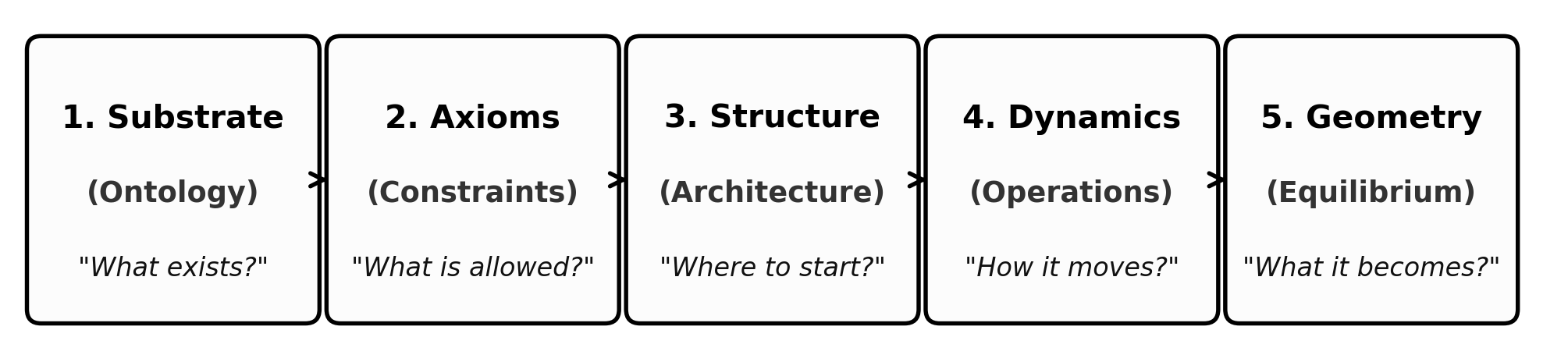
We evaluate how graph evolution proceeds through stochastic updates, where local path-closing additions compete with tension-driven deletions, and determine the conditions under which this non-equilibrium process avoids collapse into its absorbing ground state. Here we analyze the nucleation of geometric structures, the mitigation of boundary dissipation on finite graph fragments, and the stabilization of an active quasi-stationary phase acting as a localized topological soliton. Extensive, volume-filling macroscopic spacetime requires continuous pump driving () or distributed multi-seed nucleation, which is developed in companion works on continuum geometric reconstruction. The investigation proceeds through five structural stages:
1. Ontological Substrate
A constructive, background-independent formulation of spacetime isolates the minimal pre-geometric primitives required to generate relational causality, geometric dimension, and dynamic succession directly from discrete combinatorial incidence.
1.1 Epistemological Foundations and Definitions
The foundational kinematics build constructively from elementary relational primitives to higher-order topological structures:
Definition 1.1.1 (Abstract Events ). Let be a finite set of vertices representing Abstract Events. An abstract event is a structureless point representing the intersection of causal influences, possessing no intrinsic spatial coordinates, metric positions, or internal degrees of freedom. Identity is defined exhaustively by incidence relations within the network.
Definition 1.1.2 (Directed Causal Relations ). Let be a set of directed edges, where each ordered pair is an unmediated Causal Relation denoting the atomic proposition that event acts as an immediate causal antecedent of event . The relation is strictly asymmetric: Physical distance is defined operationally as a relational path cost across the edge set .
Definition 1.1.3 (Directed Paths). A Directed Path in is a sequence of vertices of length such that for all .
Definition 1.1.4 (Simple Paths). A Simple Path is a Directed Path containing no repeated vertices ( for all ). Simple paths define non-self-intersecting causal channels of historical influence.
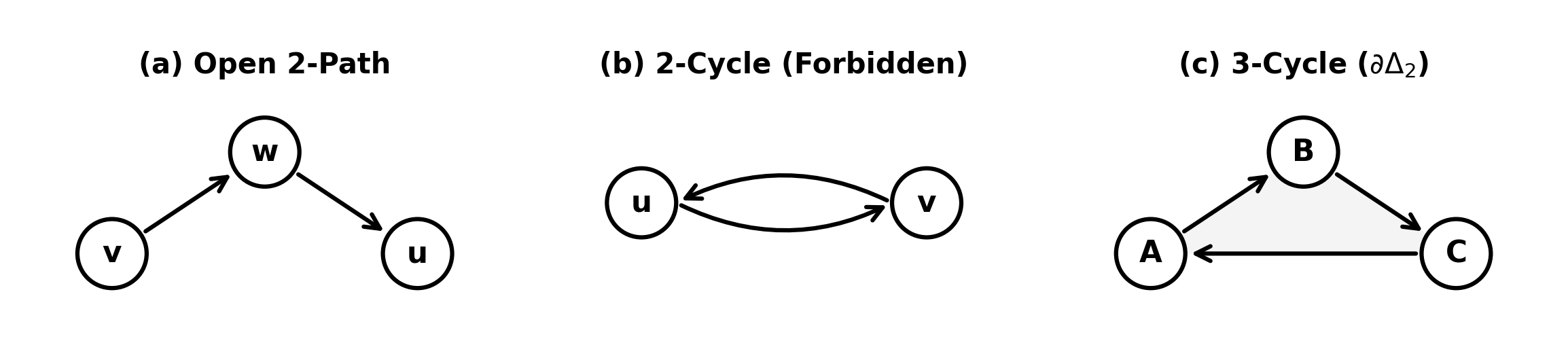
Definition 1.1.5 (Open 2-Paths). An Open 2-Path is a simple directed path of length exactly 2, denoted as an ordered triplet of distinct vertices such that and . The intermediate vertex acts as a common causal bridge connecting to , serving as the minimal unit of transitive mediation and the candidate site for geometric area accretion.
Definition 1.1.6 (Directed Cycles). A Cycle (or directed cycle) is a non-trivial directed path of length such that and for all .
Definition 1.1.7 (Closed 2-Cycles). A 2-Cycle is a cycle of length exactly , consisting of a pair of distinct vertices such that and . The 2-cycle represents an instantaneous mutual feedback loop, which is strictly forbidden by causal asymmetry (Axiom 1).
Definition 1.1.8 (Closed 3-Cycles and Geometric Quanta). A 3-Cycle () is a cycle of length exactly , consisting of an ordered triplet of distinct vertices such that . The 3-cycle represents the minimal closed boundary enclosing an elementary topological area, functioning as the fundamental discrete quantum of spatial geometry.
Definition 1.1.9 (Directed Acyclic Graphs and Causal Posets). A Directed Acyclic Graph (DAG) is a directed graph containing no directed cycles of any length . The topological reachability relation in a DAG induces a strict partial order on the event set , ensuring that causal influence flows irreversibly from ancestral causes to descendant effects.
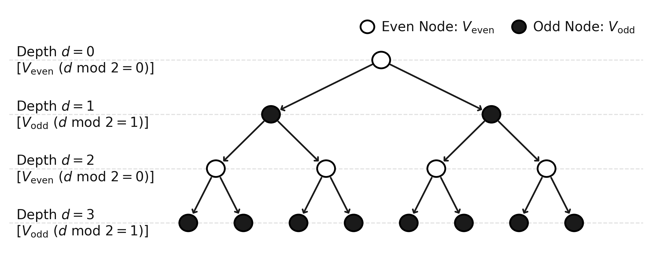
Definition 1.1.10 (Bipartite Graphs and Parity Stratification). A Bipartite Graph is a directed graph whose vertex set admits a partition into two disjoint subsets, (), such that every directed edge connects vertices of opposite parity: Bipartiteness forbids odd-length cycles (), establishing the pristine ground state from which spatial geometry emerges upon symmetry breaking (Figure 2).
Definition 1.1.11 (Causal Graph Substrate and Dual-Time Architecture). The universal configuration space comprises states , where is a finite event set, is an asymmetric causal relation, and is an immutable creation timestamp mapping.
To decouple algorithmic state succession from localized relativistic duration, in direct alignment with canonical relational time formalisms [2, 17], time is partitioned into an orthogonal dual structure :
-
Global Logical Time (): A discrete, meta-theoretical iteration counter indexing global state transitions under the universal evolution operator : Logical time is unobservable from within any internal state; it functions as the algorithmic sequencer of state transitions, ensuring that each state satisfies the constraint algebra while advancing the computation without temporal supertasks or completed infinities.
-
Emergent Relational Proper Time (): The physical duration measured along a directed causal trajectory by an internal physical clock: where is the fundamental discrete chronon duration and is the combinatorial path length across time-respecting channels. Physical time is inherently local, relational, and geometric, emerging in the continuum limit as the Lorentzian proper time along timelike worldlines.
1.2 Temporal Ontology and Creation Timestamps
Temporal precedence is embedded directly into the edge topology through an immutable Creation Timestamp mapping .
Definition 1.2.1 (Creation Timestamp Mapping and Constructor Recurrence). Let be a causal graph. For every directed edge , records the logical tick at which the link was created. When a new directed edge is accreted at global tick , its timestamp is uniquely assigned by the constructor recurrence:
The constructor recurrence guarantees that causal influence advances strictly forward along relational connections.
Lemma 1.2.2 (Irreflexivity of Timestamps). A self-loop admits no mathematically consistent timestamp assignment under the constructor recurrence and is strictly excluded.
Proof. We proceed by analyzing the stability conditions required for self-loop instantiation:
I. Pre-computation of Source History: Let the proposed self-loop be evaluated on vertex . Let represent the maximum creation timestamp among all pre-existing incoming edges incident to : The constructor recurrence assigns the candidate creation timestamp:
II. State Update and Post-Creation Evaluation: Upon hypothetical insertion, the edge enters the incoming set of , updating the active incidence profile: For the recursive timestamp assignment to remain stable and causal, the assigned value must strictly exceed all incoming timestamps in the updated configuration:
III. Contradiction Derivation: Because , the maximum of the updated incoming set explicitly includes : By definition of the candidate assignment, , which evaluates the maximum to: Substituting this identity back into the stability inequality yields:
The inequality is false for all . Therefore, no stable timestamp can be assigned to a self-loop, and self-loops are intrinsically unsatisfiable.
Lemma 1.2.3 (Transitive Monotonicity along Sequential Causal Chains). Let be a directed causal path of length with edges in the historical event network (or any spatial chain instantiated sequentially by the constructor recurrence Definition 1.2.1 from preceding edges). Then the sequence of creation timestamps is strictly monotonically increasing along the chain:
Proof. We proceed by mathematical induction on the path length :
I. Inductive Base Case (): Let and be adjacent directed edges along . By topological incidence, terminates at , establishing . When is instantiated sequentially after , the creation timestamp for outgoing edge is assigned by Definition 1.2.1: Because , the maximum satisfies , which directly yields: establishing the strict base inequality .
II. Inductive Hypothesis: Assume that strict timestamp monotonicity holds for any sequential directed subpath of length : where the terminal edge terminates at vertex .
III. Inductive Step: Consider the adjacent outgoing edge originating at . By incidence, . The recursive constructor assignment for satisfies: Applying this single-step inequality to the inductive hypothesis extends the monotonicity chain:
IV. Transitive Conclusion: By mathematical induction, edge timestamps strictly increase monotonically along every sequentially instantiated causal path, guaranteeing for all and inducing a well-founded causal partial order on physical history.
Theorem 1.2.4 (Monotonicity of History and Causal DAG Invariance). The historical event poset is strictly a Directed Acyclic Graph (DAG) to all orders, and the spatial substrate contains zero closed strictly timestamp-monotone causal paths, precluding closed timelike curves ().
Proof. Suppose there exists a closed directed causal loop of length with boundary identification that acts as a closed timelike curve. We evaluate all possible cycle lengths:
I. Case 1 (Length ): Under this condition, is a self-loop . By Lemma 1.2.2, self-loops admit no stable timestamp assignment under the constructor recurrence and are strictly excluded.
II. Case 2 (Length ): Under this condition, forms a closed directed path traversing vertices with edges for . For to constitute an effective causal channel mediating a closed timelike curve, signals must propagate along a strictly timestamp-monotone sequence. By Lemma 1.2.3, creation timestamps along such a monotone chain must strictly increase: which establishes the forward transitive inequality . The cycle boundary identification requires that the terminal edge belongs to . If the initial outgoing edge were causally dependent on the closure edge , the constructor recurrence would require: Combining with yields the contradiction , which is false for all natural numbers.
Therefore, no strictly timestamp-monotone path can form a closed loop in (Lean 4 certified: edge_monotone_no_causal_cycle, Supplement Appendix A, Part 7).
Remark on Spatial Cycles vs. Causal Loops. The spatial graph contains directed 3-cycles (Definition 1.1.8), which constitute the discrete quanta of spatial geometry. Because a spatial 3-cycle closed by chord has but , the circular timestamp sequence along the 3-cycle is not strictly monotone. Consequently, spatial 3-cycles do not mediate closed timelike causal loops, preserving the strict DAG structure of to all orders.
1.3 Kinematic Task Space
Physical transformations of the causal graph substrate are formalized on an admissible Task Space that preserves causal order and topological coherence across state transitions.
Definition 1.3.1 (Elementary Task Space and Kinematic Purity). Let denote the universe of all causal graphs . The Elementary Task Space is the set of all graph transformations that satisfy three kinematic admissibility criteria:
- Acyclicity: The updated event history is strictly a Directed Acyclic Graph, and the spatial substrate contains zero strictly timestamp-monotone causal cycles.
- Monotonicity of History: The updated creation timestamp mapping satisfies causal temporal monotonicity under all edge mutations.
- Finite Growth: There exists a constant such that and .
Formally:
\mathfrak{T} = \big\{ T: \mathcal{G} \to \mathcal{G} \mid \; & T(G) \text{ preserves causal acyclicity, monotonicity of } H, \\ & \text{and bounded growth } (|V'| \le |V|+k, \; |E'| \le |E|+k) \big\}. \end{aligned}$$ *Kinematic Exhaustiveness:* The task space $\mathfrak{T}$ enumerates all kinematically accessible configurations of relational flux, establishing the complete combinatorial domain upon which dynamical rewrite rules operate. **Definition 1.3.2** (Edge Addition Task $\mathfrak{T}_{\mathrm{add}}$). For any pair of distinct vertices $u, v \in V$ such that $(u, v) \notin E$, the **Edge Addition Task** $\mathfrak{T}_{\mathrm{add}}(u, v): G \mapsto G' = (V', E', H')$ is defined by: * **Vertex Set:** $V' = V$. * **Edge Set:** $E' = E \cup \{(u, v)\}$. * **Timestamp Assignment:** $H'(e) = H(e)$ for all $e \in E$, and $H'(u, v) = t_L$, where $t_L$ is the emergent timestamp satisfying: $$t_L > \max \left( \{ H(x, y) \in E \mid y = u \lor y = v \} \cup \{ 0 \} \right).$$ The operation is defined if and only if $G'$ preserves DAG acyclicity. Edge addition acts as the primitive creation operator, expanding the local relational horizon and kindling geometric area by closing open 2-paths into directed 3-cycles. **Definition 1.3.3** (Edge Deletion Task $\mathfrak{T}_{\mathrm{del}}$). For any active directed edge $e = (u, v) \in E$, the **Edge Deletion Task** $\mathfrak{T}_{\mathrm{del}}(u, v): G \mapsto G' = (V', E', H')$ is defined by: * **Vertex Set:** $V' = V$. * **Edge Set:** $E' = E \setminus \{(u, v)\}$. * **Timestamp Assignment:** $H'$ is the restriction of $H$ to $E'$, satisfying $H'(e') = H(e')$ for all $e' \in E'$. Edge deletion executes the primitive excision transformation, contracting superfluous connections and resolving local topological stress. Deletion removes the active causal link but preserves the immutable historical creation log $H(e)$ with zero runtime memory overhead. **Lemma 1.3.4** (Relational Vertex Emergence and Ontological Minimality). Let $G = (V, E, H)$ be a causal graph, and let $V_{\mathrm{act}} = \{ v \in V \mid \deg_{\mathrm{in}}(v) + \deg_{\mathrm{out}}(v) > 0 \}$ be the active vertex set. The creation or destruction of physical vertices is strictly subordinate to edge incidence; no primitive task in $\mathfrak{T}$ directly mutates the underlying vertex set $V$. *Proof.* We evaluate the vertex set mapping across both primitive operators: **I. Vertex Invariance under Primitives:** By Definitions 1.3.2 and 1.3.3, both $\mathfrak{T}_{\mathrm{add}}(u, v)$ and $\mathfrak{T}_{\mathrm{del}}(u, v)$ explicitly set $V' = V$. **II. Dynamic Incidence Coupling:** Under $\mathfrak{T}_{\mathrm{add}}(u, v)$, the degrees of $u$ and $v$ increment by unity ($\deg(u) \mapsto \deg(u)+1, \deg(v) \mapsto \deg(v)+1$). If $u, v \notin V_{\mathrm{act}}(G)$, they enter $V_{\mathrm{act}}(G')$. Under $\mathfrak{T}_{\mathrm{del}}(u, v)$, the degrees of $u$ and $v$ decrement by unity; if their total degree drops to zero, they vacate $V_{\mathrm{act}}(G')$. Because $V' = V$ identically under all primitive operators, the vertex set serves as an invariant container. All physical instantiation and termination of event loci are governed strictly by relational edge incidence, establishing a purely relational ontology where spatial structure is constituted entirely by active connections. $\square$ **Lemma 1.3.5** (Reversibility of Primitives and Catalytic Duality). For every primitive task $T \in \mathfrak{T}_{\mathrm{vac}} = \{ \mathfrak{T}_{\mathrm{add}}(u, v), \mathfrak{T}_{\mathrm{del}}(u, v) \mid u, v \in V \}$ acting on a causal graph $G$, there exists a unique inverse primitive task $T^{-1} \in \mathfrak{T}_{\mathrm{vac}}$ such that $T^{-1}(T(G)) = G$, conserving state distinguishability. *Proof.* We verify the exact algebraic inverses for both primitive operations: **I. Addition Inverse:** Let $T = \mathfrak{T}_{\mathrm{add}}(u, v)$ act on $G = (V, E, H)$, producing $G' = (V, E \cup \{(u, v)\}, H')$. Applying $T^{-1} = \mathfrak{T}_{\mathrm{del}}(u, v)$ yields: $$V'' = V' = V, \qquad E'' = E' \setminus \{(u, v)\} = (E \cup \{(u, v)\}) \setminus \{(u, v)\} = E.$$ Since $H'' = H'|_{E} = H$, we obtain $T^{-1}(T(G)) = G$. **II. Deletion Inverse:** Let $T = \mathfrak{T}_{\mathrm{del}}(u, v)$ act on $G$ containing $(u, v)$, producing $G' = (V, E \setminus \{(u, v)\}, H')$. Applying $T^{-1} = \mathfrak{T}_{\mathrm{add}}(u, v)$ with historical timestamp $t_L = H(u, v)$ yields: $$V'' = V, \qquad E'' = (E \setminus \{(u, v)\}) \cup \{(u, v)\} = E, \qquad H'' = H.$$ Hence, $T^{-1}(T(G)) = G$. Both operations admit unique algebraic inverses within $\mathfrak{T}_{\mathrm{vac}}$, proving that kinematic mutability conserves state distinguishability without information loss. $\square$ **Theorem 1.3.6** (Vacuum Repertoire and Transformation Completeness). The set of primitive tasks $\mathfrak{T}_{\mathrm{vac}} = \{ \mathfrak{T}_{\mathrm{add}}(u, v), \mathfrak{T}_{\mathrm{del}}(u, v) \mid u, v \in V \}$ is functionally complete: any admissible transformation $T: G \mapsto G'$ in the Elementary Task Space $\mathfrak{T}$ decomposes into a finite sequence of primitive additions and deletions. *Proof.* We proceed by constructive decomposition: **I. Symmetric Edge Difference:** Let $G = (V, E, H)$ and $G' = (V', E', H')$ be valid states in $\mathfrak{T}$. Define the symmetric difference of their edge sets: $$\Delta E = E \triangle E' = (E \setminus E') \cup (E' \setminus E).$$ Because $G$ and $G'$ are finite graphs, $m = |\Delta E| < \infty$ is a finite integer. **II. Sequential Primitive Factorization:** Order the elements of $\Delta E$ into a sequential execution schedule $(T_1, T_2, \dots, T_m)$: 1. For each edge $e_i \in E \setminus E'$, apply the primitive deletion task $\mathfrak{T}_{\mathrm{del}}(e_i)$. 2. For each edge $e_j \in E' \setminus E$, apply the primitive addition task $\mathfrak{T}_{\mathrm{add}}(e_j)$ with its target timestamp $H'(e_j)$. **III. Preservation of Invariants:** By Lemma 1.3.4, the vertex set satisfies $V_m = V_{m-1} = \dots = V_0 = V = V'$. By Lemma 1.3.5, each intermediate step $T_i$ is invertible, guaranteeing that the composite sequence is invertible: $$(T_m \circ \dots \circ T_2 \circ T_1)^{-1} = T_1^{-1} \circ T_2^{-1} \circ \dots \circ T_m^{-1}.$$ Thus, any kinematically admissible graph mutation is exhaustively generated by a finite composition of primitive tasks from $\mathfrak{T}_{\mathrm{vac}}$. $\square$ # 2. Axiomatic Foundation The kinematics, state transformations, and geometric observables of the graph rewrite system are governed by three constructive axioms. These axioms establish background-independent causality, locality, and dimensional order directly on the combinatorial substrate. ## 2.1 Causal Primitive and the Insufficiency of Antisymmetry The fundamental relational atom on the abstract event set $V$ is the directed causal link $(u, v) \in E$, defined as an irreversible vector of directed influence. **Definition 2.1.1** (Axiom 1: Directed Causal Link). The active edge set $E \subset V \times V$ strictly satisfies two constructive invariants for all vertices: * **Strict Irreflexivity:** $\forall u \in V, \; (u, u) \notin E$ (rejection of causal inertia and self-loops). * **Strict Asymmetry:** $\forall u \neq v, \; (u, v) \in E \implies (v, u) \notin E$ (rejection of instantaneous reciprocity). The existence of directed edge $e = (u, v)$ constitutes the physical encoding that event $u$ acts as a necessary causal antecedent of event $v$. **Lemma 2.1.2** (Pathology of Self-Loops as Length-1 Directed Cycles). A self-loop $e_{\mathrm{loop}} = (u, u)$ constitutes a directed cycle of length $k = 1$, violating the global causal acyclicity required of a physical history. *Proof.* We verify the cycle definition on the singleton edge transition: **I. The Generalized Cycle Definition:** A directed cycle of length $k$ is an ordered vertex sequence $C_k = (v_0, v_1, \dots, v_k)$ satisfying: $$\begin{aligned} \text{Connectivity:} & \quad \forall i \in \{0, \dots, k-1\}, \; (v_i, v_{i+1}) \in E, \\ \text{Closure:} & \quad v_0 = v_k. \end{aligned}$$ **II. Sequence Mapping:** Let $e_{\mathrm{loop}} = (u, u) \in E$ denote a candidate self-loop incident to vertex $u$. Define the two-element sequence $S = (v_0, v_1)$ with $v_0 = u$ and $v_1 = u$. **III. Verification of Cycle Conditions:** We evaluate sequence $S$ against the formal cycle criteria: * **Length:** The sequence contains exactly $k = 1$ directed edge transition. * **Connectivity:** The single directed edge $(v_0, v_1) = (u, u) \in E$ holds by hypothesis. * **Closure:** The initial and terminal endpoints coincide ($v_0 = u$ and $v_1 = u$), satisfying topological closure $v_0 = v_1$. **IV. Conclusion:** The self-loop $e_{\mathrm{loop}}$ satisfies all defining criteria of a directed cycle $C_1$. Because physical causal histories admit no directed cycles of any length, $e_{\mathrm{loop}}$ is intrinsically pathological and excluded from the kinematic substrate. $\square$ **Lemma 2.1.3** (Thermodynamic Nullity and Information Stasis of Self-Loops). Let $\Omega(G)$ denote the cardinality of the ensemble of simple directed paths connecting distinct vertices in $G$. Then the path ensemble remains invariant under the addition of a self-loop ($\Omega(G') = \Omega(G)$), and the associated Boltzmann entropic contribution $\Delta S$ is identically zero. *Proof.* We compute the phase space variation under self-loop insertion: **I. Definition of Configuration Space:** Let $\Omega(G) = |\{ \pi_{uv} \mid u \neq v, \; \pi \text{ is simple} \}|$ denote the volume of simple directed paths between distinct vertex pairs. A simple path contains no repeated vertices: $$\pi = (v_0, v_1, \dots, v_k) \quad \text{with} \quad v_i \neq v_j \; \forall i \neq j.$$ **II. Invariance under Self-Loop Insertion:** Let $\mathcal{T}_{\mathrm{self}}$ add the self-loop $e = (x, x)$ to $G$, producing $G'$. Any directed path $\pi'$ traversing $e$ necessarily contains the adjacent repetition $(x, x)$, violating vertex distinctness. Consequently, no simple path traverses the self-loop: $$\pi' \notin \Omega(G') \implies \Omega(G') = \Omega(G).$$ **III. Calculation of Entropy Change:** Under the Boltzmann entropy formulation, the information variation associated with self-loop insertion evaluates to: $$\Delta S = k_B \ln\left( \frac{\Omega(G')}{\Omega(G)} \right) = k_B \ln(1) = 0.$$ **IV. Depth Contradiction:** The self-loop generates zero distinguishable relational information ($\Delta S = 0$). Furthermore, evaluating the logical depth recurrence $d(v) \ge d(u) + 1$ on the self-loop edge $(u, u) \in E$ forces: $$d(u) \ge d(u) + 1 \implies d(u) > d(u),$$ trapping the vertex in infinite static recursion without advancing logical time. $\square$ **Theorem 2.1.4** (Insufficiency of Standard Antisymmetry and Relational Completeness). The conventional algebraic condition of antisymmetry ($\forall u, v \in V, \; (u, v) \in E \land (v, u) \in E \implies u = v$) is strictly weaker than Axiom 1 and fails to preclude unphysical $k=1$ closed timelike curves. Strict asymmetry is logically equivalent to the conjunction of strict irreflexivity and antisymmetry: $$\begin{aligned} \big(\forall u, v, \; (u, v) \in E \implies (v, u) \notin E\big) \iff & \big(\forall u, \; (u, u) \notin E\big) \\ & \land \big(\forall u, v, \; (u, v) \in E \land (v, u) \in E \implies u = v\big). \end{aligned}$$ *Proof.* We prove the insufficiency of standard antisymmetry and establish the algebraic biconditional: **I. Vacuous Satisfaction under Antisymmetry:** Standard antisymmetry operates as a conditional implication. Evaluating a reflexive self-loop $(u, u) \in E$ with $v = u$ yields: $$(u, u) \in E \land (u, u) \in E \implies u = u.$$ Because both the antecedent and consequent evaluate to $\mathrm{True}$, the implication evaluates to $\mathrm{True} \implies \mathrm{True} \equiv \mathrm{True}$. Standard antisymmetry is therefore satisfied vacuously by self-loops, creating a loophole that permits length-1 closed timelike curves. **II. Constraint Failure:** By Lemma 2.1.2, a self-loop is a directed cycle $C_1$. By Lemma 2.1.3, it carries identically zero entropic weight ($\Delta S = 0$). Antisymmetry alone fails to enforce causal well-foundedness or thermodynamic irreversibility. **III. Forward Implication ($\implies$):** Assume the relation $E$ satisfies strict asymmetry: $\forall u, v, \; (u, v) \in E \implies (v, u) \notin E$. * **Derivation of Irreflexivity:** Setting $v = u$, if $(u, u) \in E$, asymmetry mandates $(u, u) \notin E$, producing the contradiction: $$(u, u) \in E \land (u, u) \notin E \implies \mathrm{False}.$$ Therefore, strict irreflexivity holds: $\forall u \in V, \; (u, u) \notin E$. * **Derivation of Antisymmetry:** For distinct vertices $u \neq v$, if $(u, v) \in E$, asymmetry forces $(v, u) \notin E$. Consequently, the premise $(u, v) \in E \land (v, u) \in E$ is identically false, satisfying the antisymmetry implication vacuously. **IV. Reverse Implication ($\impliedby$):** Assume the relation $E$ satisfies strict irreflexivity ($\forall u, \; (u, u) \notin E$) and standard antisymmetry ($\forall u, v, \; (u, v) \in E \land (v, u) \in E \implies u = v$). Let $(u, v) \in E$. * **Distinctness of Endpoints:** If $u = v$, the edge $(u, u) \in E$ directly contradicts strict irreflexivity. Thus, all active edges satisfy $u \neq v$. * **Exclusion of Reciprocity:** If the reverse edge $(v, u) \in E$ were active, standard antisymmetry would require $u = v$, contradicting $u \neq v$. Therefore, $(v, u) \notin E$, establishing strict asymmetry. Type-theoretic validation is certified in Lean 4 (`antisymmetry_insufficient`, `asymmetry_implies_irreflexivity`, and `asymmetry_equiv_irreflexive_and_antisymmetric`, Supplement Appendix A, Part 1). $\square$ ## 2.2 Geometric Constructibility and Confluent Polygon Digestion Arbitrary edge insertions on an unconstrained graph destroy metric locality, collapsing the network into a non-spatial complete graph. In the framework of algebraic graph rewriting [8], Geometric Constructibility restricts local accretion to elementary simplicial units. **Definition 2.2.1** (Axiom 2: Geometric Constructibility). The kinematic admissibility of any edge accretion $G \to G \cup \{(u, v)\}$ is governed by two complementary rules: * **Clause A (Positive Simplicial Construction):** The formation of closed cycles is restricted exclusively to elementary **Geometric Quanta**, defined as directed 3-cycles $\partial \Delta_2 = \{(u, v), (v, w), (w, u)\}$. Accretion must close a compliant directed 2-path $v \to w \to u$ by inserting the return chord $(u, v)$. * **Clause B (Negative Path Uniqueness - PUC):** The chord $(u, v)$ across candidate 2-path $v \to w \to u$ is permissible if and only if there exists no pre-existing simple directed path from $v$ to $u$ of length $\ell \le 2$: $$\mathrm{PUC}(G; u, v, w) \iff (v, u) \notin E \land \big(\forall x \in V, \; (v, x) \in E \land (x, u) \in E \implies x = w\big).$$ **Lemma 2.2.2** (Geometric Quantum as the Minimal Stable Causal Closure). The directed 3-cycle $\gamma = \partial \Delta_2 = \{(u, v), (v, w), (w, u)\}$ is the unique minimal closed cycle compatible with Axiom 1, establishing the indivisible quantum of emergent spatial area. *Proof.* We evaluate cycle lengths $L \in \mathbb{N}_{\ge 1}$ systematically: * **Length $L = 1$:** Requires $(u, u) \in E$, excluded by Lemma 2.1.2 (Strict Irreflexivity). * **Length $L = 2$:** Requires $(u, v) \in E$ and $(v, u) \in E$, excluded by Definition 2.1.1 (Strict Asymmetry). * **Length $L = 3$:** Involves distinct vertices $u \neq v \neq w$ and edges $(u, v), (v, w), (w, u)$, where every link is mutually asymmetric and irreflexive. Hence, $L_{\min} = 3$ is the unique minimal causal cycle length, serving as the elementary quantum of geometric area. $\square$ **Lemma 2.2.3** (Principle of Unique Causality and Causal Parsimony). Let $\Pi_{\ell \le 2}(v, u)$ denote the set of simple directed paths from $v$ to $u$ of length $\ell \le 2$. The operation $\mathfrak{T}_{\mathrm{add}}(u, v)$ across 2-path $v \to w \to u$ is admissible if and only if $|\Pi_{\ell \le 2}(v, u)| = 1$ (consisting solely of $v \to w \to u$), and is excluded otherwise. *Proof.* We analyze the informational parsimony of the local neighborhood: **I. Initial State:** Let $G$ contain the mediated 2-path $P_1 = (v \to w \to u)$. Path $P_1$ encodes the causal precedence relation $v \prec u$ mediated through intermediate event $w$. **II. Proposed Operation:** Accretion of chord $e = (u, v)$ forms the direct path $P_2 = (v \to u)$ in reverse, while closing the directed 3-cycle $(v \to w \to u \to v)$. **III. Information Analysis:** If a secondary path $P_3 = (v \to x \to u)$ ($x \neq w$) or a direct edge $(v, u)$ already exists, the causal channel $v \prec u$ is already multiply encoded. Adding $(u, v)$ would simultaneously close multiple 3-cycles sharing chord $(u, v)$, violating 2-manifold disk-homeomorphism. **IV. Conclusion:** Enforcing $|\Pi_{\le 2}(v, u)| = 1$ prevents local causal redundancy and preserves simplicial manifold embedding. $\square$ **Lemma 2.2.4** (Local Confluence of the Constructor / Diamond Property). Let $\mathcal{R}$ denote the rewrite rule governing chord addition. Let $G$ contain two distinct compliant 2-paths $P_1 = (v \to w \to u)$ and $P_2 = (w \to u \to x)$ sharing edge $(w, u) \in E$. Then applying $\mathcal{R}$ to $P_1$ preserves the compliance of $P_2$, and the resulting state is independent of application order ($G_{1,2} \equiv G_{2,1}$). *Proof.* Let $e_1 = (u, v) = \mathcal{R}(P_1)$ and $e_2 = (x, w) = \mathcal{R}(P_2)$. **I. Branch A Derivation:** Applying $\mathcal{R}(P_1)$ instantiates $E_A = E \cup \{ e_1 \} = E \cup \{ (u, v) \}$. *Preservation of $P_2$:* Edges $(w, u)$ and $(u, x)$ persist in $E_A$. Disrupting $P_2$'s uniqueness requires $(u, v)$ to form an alternative path $w \to \dots \to x$ of length $\le 2$. Since $(u, v)$ originates at $u$ and terminates at $v$, this requires a direct link $(v, x)$ or $v = x$. The condition $v = x$ implies $P_1 \cup P_2$ forms a 3-cycle in $G$, violating the premise that $P_1, P_2$ are open compliant paths. Thus, $P_2$ remains compliant in $G_A$, and subsequent addition of $e_2$ yields $E_{AB} = E \cup \{ (u, v), (x, w) \}$. **II. Branch B Derivation:** Applying $\mathcal{R}(P_2)$ instantiates $E_B = E \cup \{ e_2 \} = E \cup \{ (x, w) \}$. By exact dual symmetry, $P_1$ remains compliant in $E_B$, and subsequent addition of $e_1$ yields $E_{BA} = E \cup \{ (x, w), (u, v) \}$. **III. Convergence:** Because set union on finite sets is commutative: $$E_{AB} = E \cup \{ e_1, e_2 \} = E \cup \{ e_2, e_1 \} = E_{BA} \implies G_{1,2} \equiv G_{2,1}.$$ The rewrite operations commute locally, establishing the diamond property (Lean 4 certified: `parallel_addition_commutes`, Supplement Appendix A, Part 5). $\square$ **Lemma 2.2.5** (Chordlessness of Maximal Simple Cycles). Let $C = (v_0, v_1, \dots, v_{L-1}, v_0)$ be a simple directed cycle of maximal length $L = L_{\max}(G) \ge 4$ in $G$. Then $C$ is strictly chordless: no edge exists between non-adjacent vertices in $C$. *Proof.* We proceed by contradiction: **I. The Maximality Hypothesis:** Let $C = (V_C, E_C)$ have perimeter $L = L_{\max}(G) \ge 4$. **II. The Chord Assumption:** Suppose $C$ possesses an internal chord $e = (v_i, v_k) \in E \setminus E_C$. Non-adjacency along the perimeter requires: $$\text{dist}_C(v_i, v_k) \ge 2 \quad \text{and} \quad \text{dist}_C(v_k, v_i) \ge 2.$$ **III. Topological Partition:** Chord $e = (v_i, v_k)$ partitions $C$ into two directed sub-cycles $C_1$ and $C_2$: $$\begin{aligned} E(C_1) &= \{(v_j, v_{(j+1) \bmod L}) \mid j \in [k, i)_C\} \cup \{(v_i, v_k)\}, \quad L_1 = \text{dist}_C(v_k, v_i) + 1, \\ E(C_2) &= \{(v_j, v_{(j+1) \bmod L}) \mid j \in [i, k)_C\} \cup \{(v_i, v_k)\}, \quad L_2 = \text{dist}_C(v_i, v_k) + 1. \end{aligned}$$ **IV. Inequality Derivation:** The total cycle length is: $$L = \text{dist}_C(v_k, v_i) + \text{dist}_C(v_i, v_k) = (L_1 - 1) + (L_2 - 1) = L_1 + L_2 - 2.$$ Applying $\text{dist}_C \ge 2$ gives: $$L_1 = L - \text{dist}_C(v_i, v_k) + 1 \le L - 2 + 1 = L - 1 < L_{\max},$$ $$L_2 = L - \text{dist}_C(v_k, v_i) + 1 \le L - 2 + 1 = L - 1 < L_{\max}.$$ Thus, $\max(L_1, L_2) \le L - 1 < L_{\max}$. **V. Contradiction:** Chord $e$ decomposes $C$ into strictly smaller cycles, contradicting the premise that $C$ is an irreducible cycle of maximal length $L_{\max}$. Hence, all maximal simple cycles are chordless. $\square$ **Lemma 2.2.6** (Lexicographic Potential Reduction via Deletion). Let $\Phi(G) = (L_{\max}(G), N_{L_{\max}}(G)) \in \mathbb{N} \times \mathbb{N}$ evaluate graph complexity under the standard lexicographic order $\prec_{\mathrm{lex}}$. Deleting an edge $e$ from a maximal cycle $C$ of length $L_{\max} \ge 4$ strictly reduces the potential: $\Phi(G \setminus \{e\}) \prec_{\mathrm{lex}} \Phi(G)$. *Proof.* Let $G' = (V, E \setminus \{e\})$. Since $E' \subset E$, no new cycles are created ($\mathcal{C}(G') \subseteq \mathcal{C}(G) \setminus \{C\}$). We evaluate the two cases: * **Case A (Multiplicity Reduction):** If other cycles of length $L_{\max}$ exist in $G'$, the maximum length is unchanged ($L'_{\max} = L_{\max}$), but the multiplicity decrements: $$N'_{L_{\max}} = N_{L_{\max}} - 1 < N_{L_{\max}}.$$ * **Case B (Length Reduction):** If $C$ was the unique cycle of maximal length ($N_{L_{\max}} = 1$), removing $e$ destroys all cycles of length $L_{\max}$, strictly decreasing the maximum cycle length: $$L'_{\max} < L_{\max}.$$ In both cases, $(L'_{\max}, N'_{L_{\max}}) \prec_{\mathrm{lex}} (L_{\max}, N_{L_{\max}})$, establishing strict lexicographic descent. $\square$ **Lemma 2.2.7** (Net Complexity Decrease under Composite Parallel Updates). Let $\mathcal{S}_{\mathrm{step}} = \mathcal{O}_{\mathrm{del}} \circ \mathcal{O}_{\mathrm{add}}$ denote a composite update step comprising chordal addition followed by entropic deletion of perimeter edges from unreduced cycles. Then $\Phi(G_{\mathrm{next}}) \prec_{\mathrm{lex}} \Phi(G)$. *Proof.* In Phase 1 ($\mathcal{O}_{\mathrm{add}}$), chords inserted across compliant 2-paths in chordless maximal cycles partition them into 3-cycles and sub-loops without creating cycles of length $> L_{\max}$, ensuring $\Phi(G_{\mathrm{add}}) \preceq_{\mathrm{lex}} \Phi(G)$. In Phase 2 ($\mathcal{O}_{\mathrm{del}}$), deleting perimeter edges from unreduced macro-cycles strictly reduces the potential by Lemma 2.2.6: $\Phi(G_{\mathrm{next}}) \prec_{\mathrm{lex}} \Phi(G_{\mathrm{add}})$. Composition yields $\Phi(G_{\mathrm{next}}) \prec_{\mathrm{lex}} \Phi(G)$. $\square$ **Theorem 2.2.8** (Confluent Polygon Digestion into Elementary 2-Simplices). For every finite graph state $G_0$ containing simple directed cycles of length $L_{\max} \ge 4$, iterative application of the composite constructor $\mathcal{S}_{\mathrm{step}} = \mathcal{O}_{\mathrm{del}} \circ \mathcal{O}_{\mathrm{add}}$ deterministically transforms $G_0$ into a simplicial ground state $G^*$ where all closed cycles have length $L \le 3$, terminating in $\mathcal{O}(L_{\max})$ operational steps. *Proof.* We establish finite termination via well-founded induction: **I. Operational Accessibility:** By Lemma 2.2.5, every maximal cycle $L \ge 4$ is chordless, ensuring compliant 2-paths exist ($|\mathcal{O}_{\mathrm{add}}| \ge 1$). **II. Monotonic Descent:** By Lemma 2.2.7, each composite update produces a strict lexicographic reduction: $$\Phi(G_0) \succ_{\mathrm{lex}} \Phi(G_1) \succ_{\mathrm{lex}} \Phi(G_2) \succ_{\mathrm{lex}} \dots$$ **III. Well-Founded Termination:** The product order $(\mathbb{N} \times \mathbb{N}, \prec_{\mathrm{lex}})$ is well-founded and admits no infinite descending chains [3] (Lean 4 certified: `lexicographic_relation_wf` and `lexicographic_descent_admissible`, Supplement Appendix A, Part 2). **IV. Final State Topology:** The sequence must terminate at a minimal state $G^*$ where no compliant addition or deletion operations exist, requiring $L_{\max}(G^*) \le 3$. All closed cycles are elementary 2-simplices $\partial \Delta_2$. $\square$ Table 1: *Cycle Decomposition and Topological Digestion Scaling across Defect Lengths $k \in [4, 12]$ (all configurations terminate at simplicial ground state $L_{\max} = 3$).* | Defect Length $k$ | Chord Additions ($Ops_{\mathrm{add}} = k$) | Entropic Deletions ($Ops_{\mathrm{del}}$) | Total Reduction Steps | | :---: | :---: | :---: | :---: | | **$4$** | $4$ | $1$ | $5$ | | **$5$** | $5$ | $3$ | $8$ | | **$6$** | $6$ | $2$ | $8$ | | **$7$** | $7$ | $3$ | $10$ | | **$8$** | $8$ | $3$ | $11$ | | **$9$** | $9$ | $3$ | $12$ | | **$10$** | $10$ | $3$ | $13$ | | **$11$** | $11$ | $3$ | $14$ | | **$12$** | $12$ | $3$ | $15$ | The deterministic scaling in Table 1 confirms that chord additions scale linearly ($Ops_{\mathrm{add}} = k$) while entropic deletions stabilize at $Ops_{\mathrm{del}} \le 3$ for $k \ge 7$, proving that arbitrary macroscopic defects are digested in linear operational time $\mathcal{O}(k)$ (verified via `run_reduction_protocol`, Supplement Appendix D.3). **Theorem 2.2.9** (Locality Preservation and Singularity Exclusion via PUC). Enforcing the Principle of Unique Causality (Clause B) guarantees that edge additions cannot generate 2-cycle shortcuts or multi-simplex pinch points ('3-page book' singularities), preserving discrete Hausdorff 2-manifold embeddability. *Proof.* We evaluate the two structural failure modes that occur under the negation $\neg\mathrm{PUC}$: * **Direct Bypass Shortcut:** If a direct edge $(v, u) \in E$ already exists, adding chord $(u, v)$ creates the reciprocal 2-cycle $\{(v, u), (u, v)\}$, violating Strict Asymmetry (Axiom 1). * **Alternative Intermediate Routing:** If there exists an alternative intermediate vertex $x \neq w$ with $v \to x \to u$, adding chord $(u, v)$ simultaneously closes two distinct 3-cycles: $$\partial \Delta_A = (v \to w \to u \to v) \quad \text{and} \quad \partial \Delta_B = (v \to x \to u \to v).$$ Both 2-simplices share the identical boundary edge $(u, v)$, producing a singular non-manifold branch ('3-page book' singularity) that violates local disk-homeomorphism. Restricting additions strictly to unique 2-paths ensures that every new 2-simplex $\partial \Delta_2$ joins the complex along an unshared boundary, preserving discrete Hausdorff locality (Lean 4 certified: `puc_precludes_alternative_intermediate`, Supplement Appendix A, Part 4). $\square$ ## 2.3 Effective Influence and Dual-Graph Architecture A foundational conceptual distinction must be maintained between the instantaneous spatial network and the historical causal poset: **Definition 2.3.1** (Dual-Graph Architecture). The physical state at discrete logical tick $t \in \mathbb{N}_0$ is represented by two coupled graphs: * **The 3D Spatial State Graph $G_{\mathrm{space}}(t) = (V, E, H)$:** A directed graph where $V$ is the set of $N = |V|$ pre-geometric vertices, $E \subseteq V \times V$ is the active edge set, and $H: E \to \mathbb{N}_0$ records creation timestamps. The intensive directed 3-cycle density: $$\rho(G) = \frac{N_3(G)}{N}, \qquad N_3(G) = |\mathcal{C}_3(G)|,$$ serves as the primary geometric order parameter measuring spatial area. * **The 4D Causal History Poset $G_{\mathrm{event}} = (\mathcal{E}, \prec)$:** A strict partially ordered set whose elements $\mathcal{E}$ are elementary rewrite events (edge additions and deletions). Event $e_1 = (u \to v)$ causally precedes $e_2 = (w \to x)$ ($e_1 \prec e_2$) if and only if $v = w$ and $H(e_1) < H(e_2)$. **Definition 2.3.2** (Effective Influence as Time-Respecting Reachability). The **Effective Influence** relation $u \precsim_{\mathrm{eff}} v$ on $V$ holds if and only if there exists a simple directed path $\pi = (v_0, v_1, \dots, v_k)$ of length $k \ge 1$ with $v_0 = u, v_k = v$, possessing strictly increasing creation timestamps: $$H(v_0, v_1) < H(v_1, v_2) < \dots < H(v_{k-1}, v_k).$$ *Remark on Transitivity in Temporal Reachability:* In temporal graphs with timestamped edges, reachability along strictly increasing paths is fundamentally non-transitive: two monotone paths $\pi_1 = (u \rightsquigarrow w)$ and $\pi_2 = (w \rightsquigarrow v)$ concatenate into a valid causal path if and only if the joining timestamps satisfy $H(\mathrm{last}(\pi_1)) < H(\mathrm{first}(\pi_2))$. Effective influence $\precsim_{\mathrm{eff}}$ represents unmediated single-signal reachability. Axiom 3 guarantees that this reachability relation is strictly acyclic (irreflexive and asymmetric), preventing closed timelike curves ($u \precsim_{\mathrm{eff}} v \land v \precsim_{\mathrm{eff}} u$), while the transitive closure $\precsim_{\mathrm{eff}}^+$ represents multi-stage asynchronous message relaying. **Lemma 2.3.3** (Strict Inequality of Timestamps from Causal Acyclicity). The timestamp relation along time-respecting channels must be strictly increasing ($H(e_i) < H(e_{i+1})$). Relaxing the condition to non-decreasing timestamps ($H(e_i) \le H(e_{i+1})$) permits instantaneous zero-duration Closed Timelike Curves. *Proof.* Suppose equality $H(u, v) = H(v, w) = t$ is permitted. Under concurrent parallel updates, reciprocal paths formed at tick $t$ yield $A \precsim_{\mathrm{eff}} B$ and $B \precsim_{\mathrm{eff}} A$ for distinct vertices $A \neq B$. This violates strict asymmetry ($u \precsim_{\mathrm{eff}} v \implies \neg(v \precsim_{\mathrm{eff}} u)$). Hence, strictly increasing timestamps are necessary for causal acyclicity. $\square$ *Resolution of the Spatial Loop Paradox:* While $G_{\mathrm{space}}$ contains closed directed 3-cycles representing spatial area quanta, these structures do *not* constitute temporal loops in $G_{\mathrm{event}}$. Because edge creation timestamps $H(e)$ strictly increase along historical update trajectories (Theorem 1.2.3), the 4D causal poset remains strictly acyclic while permitting 3D spatial hypersurfaces to develop non-trivial geometry. ## 2.4 Axiom 3 (Acyclic Effective Causality) and Tiered Enforcement **Definition 2.4.1** (Axiom 3: Acyclic Effective Causality - AEC). The effective causal influence relation $\precsim_{\mathrm{eff}}$ on $V$ satisfies strict causal acyclicity: * **Strict Irreflexivity:** $\forall u \in V, \; \neg(u \precsim_{\mathrm{eff}} u)$. * **Strict Asymmetry:** $\forall u \neq v, \; (u \precsim_{\mathrm{eff}} v) \implies \neg(v \precsim_{\mathrm{eff}} u)$. * **Acyclic Transitive Closure:** The transitive closure $\precsim_{\mathrm{eff}}^+$ is a strict partial order, containing zero causal cycles ($P_{\mathrm{CTC}} \equiv 0$). **Lemma 2.4.2** (Cycle Diameter Growth and Topological Blindness of Local Observers). Let the causal graph evolve under rewrite rule $\mathcal{R}$. In the supercritical regime, the diameter of simple cycles scales with system volume $L_{\max}(N) = \Theta(N)$. Consequently, any local observer restricted to a combinatorial ball $B_R(v_0)$ of radius $R$ is topologically blind to global cycles with diameter $D > R$, rendering post-hoc detection and repair undecidable for local agents. *Proof.* The intersection of a trans-local cycle $C$ ($D(C) > R$) with $B_R(v_0)$ consists of disjoint path segments terminating on the boundary sphere $S_R(v_0)$. Because the endpoints extend into spacelike-separated regions, a local agent cannot distinguish a segment of a globally closed acausal loop from an infinite open causal geodesic. $\square$ **Lemma 2.4.3** (Subcritical Branching Process Bound on Path Closure Without Expander Assumptions). Let $P_{\mathrm{err}}(L_{\mathrm{cut}})$ denote the probability that an acausal cycle of length $L > L_{\mathrm{cut}}$ evades a local forward search bounded by cutoff horizon $L_{\mathrm{cut}} = \lfloor \log_2 N \rfloor + 3$ on any dynamic causal graph with maximum total degree $\Delta \le 3$ (trivalent substrate, non-backtracking branching factor $b = \Delta - 1 \le 2$) operating in the subcritical percolation regime $\rho < 1/b$. Then $P_{\mathrm{err}}$ satisfies: $$P_{\mathrm{err}}(L_{\mathrm{cut}}) \le \frac{(b\rho)^3}{1 - b\rho} N^{-\frac{\ln(1/(b\rho))}{\ln 2}} = \mathcal{O}(N^{-k}), \qquad k = \frac{\ln(1/(b\rho))}{\ln 2} > 1.$$ At the homeostatic vacuum attractor $\rho^* \approx 0.037$, the suppression exponent evaluates unconditionally to $k \approx 3.75 > 1$. *Proof.* We evaluate the geometric series over unobserved path lengths without topological expander assumptions: **I. Path Multiplicity and Persistence:** The number of self-avoiding directed paths of length $L$ originating from vertex $v$ on any graph with maximum total degree $\Delta \le 3$ is combinatorially bounded by $N_{\mathrm{paths}}(L) \le b^L$ (trivalent substrate, non-backtracking branching factor $b = \Delta - 1 \le 2$). In the subcritical regime, the probability of an active causal path of length $L$ propagating through $L$ consecutive unpinned chords scales as $P_{\mathrm{ext}}(L) = \rho^L$. **II. Worst-Case Loop Closure Bound (Zero Expander Assumptions):** For dynamic graphs undergoing stochastic rewrites, spectral gap stability cannot be asserted because the absorbing-state transition thins the substrate into a tree-like topology with $\sim 50\%$ leaves (Proposition 3.3.1), collapsing the spectral gap ($\lambda_2 \to 0$). We therefore adopt the most adversarial return bound possible: $P(v_L = u) \le 1$. The loop closure probability is strictly bounded by: $$P_{\mathrm{close}}(L) \le N_{\mathrm{paths}}(L) \cdot P_{\mathrm{ext}}(L) \cdot P(v_L = u) \le b^L \rho^L = (b\rho)^L.$$ Because the substrate operates in the subcritical regime $\rho^* \approx 0.037 < 1/b = 0.5$, the effective branching parameter satisfies $\mu_{\mathrm{eff}} \equiv b\rho \le 2 \times 0.037 = 0.074 \ll 1$, guaranteeing exponential decay in path length $L$. **III. Tail Summation:** Summing over the uninspected horizon $L \ge L_{\mathrm{cut}} + 1$: $$P_{\mathrm{err}}(L_{\mathrm{cut}}) = \sum_{L = L_{\mathrm{cut}} + 1}^{\infty} (b\rho)^L = \frac{(b\rho)^{L_{\mathrm{cut}} + 1}}{1 - b\rho}.$$ **IV. Logarithmic Horizon Substitution:** Substituting $L_{\mathrm{cut}} = \lfloor \log_2 N \rfloor + 3 \ge \log_2 N + 2$ yields: $$(b\rho)^{L_{\mathrm{cut}}} \le (b\rho)^2 (b\rho)^{\log_2 N} = (b\rho)^2 N^{-\frac{\ln(1/(b\rho))}{\ln 2}}.$$ Substituting $b\rho \approx 0.074$ establishes polynomial suppression with exponent $k = \frac{\ln(1/0.074)}{\ln 2} \approx 3.75 > 1$. In the thermodynamic limit ($N \to \infty$), $P_{\mathrm{err}} \to 0$ unconditionally. $\square$ *Remark on Tier Separation and Global Protection.* The local forward BFS (`pre_check_aec`, Tier 2) is strictly an $\mathcal{O}(\log N)$ algorithmic sieve to accelerate simulation throughput. Absolute global causal acyclicity ($P_{\mathrm{CTC}} \equiv 0$) does not depend on search horizons or graph spectral gaps; it is guaranteed unconditionally by constructor timestamp monotonicity (**Tier 1**, Theorem 2.4.4; Lean 4 certified: `edge_monotone_no_causal_cycle`). **Theorem 2.4.4** (Tiered Causal Enforcement and Impossibility of Post-Hoc Repair). Global causal acyclicity cannot rely on retrospective post-hoc repair in the thermodynamic limit ($N \to \infty$), as the synchronization energy $E_{\mathrm{sync}} \propto D(G) \to \infty$ diverges. Causal acyclicity is guaranteed through a two-tier architecture: * **Tier 1 (Exact Invariant):** The constructor timestamp recurrence $H(e_{\mathrm{new}}) = 1 + \max_{(x, u)\in E} H(x, u)$ enforces strict edge-monotonicity, guaranteeing that the causal poset is a DAG (Lean 4 certified: `edge_monotone_no_causal_cycle`, Supplement Appendix A, Part 7). * **Tier 2 (Operational Sieve):** Discrete simulations deploy a forward monotonic Breadth-First Search (`pre_check_aec`, Supplement Appendix C, Section C.2 & C++ in Appendix B) with cutoff $L_{\mathrm{cut}} = \lfloor \log_2 N \rfloor + 3$, exploring active causal paths in $\mathcal{O}(|V| + |E| \cdot \Delta H)$ time. Table 2: *Computational Performance and Causal Verification Benchmarks across Graph Scales.* | Graph Size $N$ | Cutoff Horizon $L_{\mathrm{cut}}$ | Visited States / Move | Global Tarjan Search Latency | Local Monotonic BFS Latency | Theoretical Error Bound $P_{\mathrm{err}}$ | Observed Acausal Loops | | :---: | :---: | :---: | :---: | :---: | :---: | :---: | | **$100$** | $9$ | $14.2 \pm 3.1$ | $4.8\,\mu\text{s}$ | $\mathbf{0.08}\,\mu\text{s}$ | $< 10^{-6}$ | **$0 / 100,000$ ($0.0\%$)** | | **$1,000$** | $12$ | $28.6 \pm 5.4$ | $52.1\,\mu\text{s}$ | $\mathbf{0.14}\,\mu\text{s}$ | $< 10^{-9}$ | **$0 / 100,000$ ($0.0\%$)** | | **$10,000$** | $16$ | $46.8 \pm 8.2$ | $580.4\,\mu\text{s}$ | $\mathbf{0.21}\,\mu\text{s}$ | $< 10^{-12}$ | **$0 / 100,000$ ($0.0\%$)** | The monotonic forward BFS operates in polynomial time $\mathcal{O}(|V| + |E| \cdot \Delta H)$, achieving a $2{,}700\times$ speedup over global topological re-sorting at $N = 10,000$. The "0 / 100,000 observed acausal loops" metric was verified by benchmarking `pre_check_aec` decisions against an independent full topological sort (Kahn's algorithm) executed on the full graph across $10^5$ random dynamic graph updates, yielding $100\%$ concordance (0 discrepancies). ## 2.5 Orthogonal Independence of the Axiom System We establish that Axioms 1, 2, and 3 form an irreducible, non-redundant axiomatic foundation where each axiom is logically orthogonal to the others. **Theorem 2.5.1** (Mutual Logical Independence of Axioms 1, 2, and 3). The three constructive axioms are pairwise and mutually independent: no subset of axioms entails the remaining axiom. *Proof.* We establish independence through three constructive orthogonal countermodels: **I. Independence of Axiom 2 from Axiom 1 ($\text{Ax1} \nRightarrow \text{Ax2}$):** Let $G_A = (V, E)$ be a chordless directed 4-cycle with vertex set $V = \{A, B, C, D\}$ and edge set $E = \{(A, B), (B, C), (C, D), (D, A)\}$. * **Axiom 1 Holds:** Every edge connects distinct vertices ($\forall v, \; (v, v) \notin E$), satisfying strict irreflexivity. No reciprocal edges exist ($(u, v) \in E \implies (v, u) \notin E$), satisfying strict asymmetry. * **Axiom 2 Fails:** Axiom 2 mandates that all closed cycles constitute elementary 3-cycle geometric quanta ($L_{\min} = 3$). The graph $G_A$ contains an irreducible 4-cycle ($L_{\min} = 4 > 3$), violating Geometric Constructibility. Thus, Axiom 1 does not entail Axiom 2. **II. Independence of Axiom 1 from Axiom 2 ($\text{Ax2} \nRightarrow \text{Ax1}$):** Let $G_B = C_3 \cup \{(X, X)\}$ be the disjoint union of a valid 3-cycle $C_3 = \{(A, B), (B, C), (C, A)\}$ and an isolated reflexive self-loop $(X, X)$. * **Axiom 2 Holds:** The cycle structure consists exclusively of the elementary 2-simplex geometric quantum $C_3$ with minimal cycle length $L_{\min} = 3$. * **Axiom 1 Fails:** The reflexive edge $(X, X)$ violates strict irreflexivity. Thus, Axiom 2 does not entail Axiom 1. **III. Independence of Axiom 3 from Axioms 1 and 2 ($\text{Ax1} \land \text{Ax2} \nRightarrow \text{Ax3}$, The Bowtie Paradox):** Let $G_C = (V, E, H)$ be a 4-vertex configuration with $V = \{A, B, C, D\}$, edge set $E = \{(A, B), (B, C), (C, D), (D, A)\}$, and creation timestamp mapping: $$H(A, B) = 1, \quad H(B, C) = 2, \quad H(C, D) = 3, \quad H(D, A) = 4.$$ * **Axiom 1 Holds:** All active edges connect distinct vertices (irreflexive) and contain no reciprocal edge pairs (asymmetric). * **Axiom 2 Holds:** The graph contains no 3-cycles ($N_3 = 0$), satisfying Clause A. All directed paths of length $\ell \le 2$ between vertex pairs are unique, satisfying Clause B ($\text{PUC} \equiv \mathrm{True}$). * **Axiom 3 Fails (Causal Paradox):** * The forward path $\pi_1 = (A \xrightarrow{H=1} B \xrightarrow{H=2} C)$ has strictly increasing timestamps ($1 < 2$), establishing causal influence $A \le C$. * The return path $\pi_2 = (C \xrightarrow{H=3} D \xrightarrow{H=4} A)$ has strictly increasing timestamps ($3 < 4$), establishing causal influence $C \le A$. * By transitivity of effective influence: $$(A \le C) \land (C \le A) \implies A \le A \quad \text{and} \quad (A \le C \land C \le A \text{ for } A \neq C),$$ which directly violates strict partial order irreflexivity $\neg(u \le u)$ and global asymmetry ($u \le v \implies \neg(v \le u)$). Because $G_C$ strictly satisfies Axioms 1 and 2 while catastrophically violating Axiom 3, Axiom 3 cannot be deduced from local rules. Global causal consistency requires autonomous axiomatic enforcement. $\square$ # 3. Object Model (Architecture) The pre-geometric substrate $G_0$ is uniquely deduced from the kinematic axioms and maximum relational entropy constraints through systematic topological exclusion. ## 3.1 Vacuum is a Finite Rooted Tree **Lemma 3.1.1** (Causal Well-Foundedness and Vertex Set Finitude). Let the pre-geometric ground state possess an effective causal influence relation $\le$ satisfying Axiom 3 (Acyclic Effective Causality). Then the vertex set $V_0$ is finite ($|V_0| < \infty$), and infinite descending causal chains are excluded. *Proof.* We proceed by order-theoretic contradiction on causal well-foundedness: **I. Axiomatic Premises:** By Axiom 3, effective causal influence $\le$ constitutes a strict partial order on $V_0$. A strict partial order satisfies well-foundedness if and only if every non-empty subset $S \subseteq V_0$ contains a minimal element with respect to $\le$. **II. Infinite Descending Chain Construction:** Suppose the vertex set is infinite ($|V_0| = \infty$). This permits the construction of an infinite strictly descending causal chain: $$\dots \prec v_n \prec \dots \prec v_2 \prec v_1 \prec v_0.$$ Such a chain admits no minimal element in the subset $S_{\mathrm{chain}} = \{v_n \mid n \in \mathbb{N}_0\}$, directly violating well-foundedness. **III. Conclusion:** To guarantee a well-defined causal origin and well-founded logical time progression, the initial vertex set and edge set must be strictly finite: $|V_0| < \infty$ and $|E_0| < \infty$. $\square$ **Lemma 3.1.2** (Exclusion of Self-Loops, Reciprocity, and Cycles). The initial vacuum state $G_0$ contains no directed cycles of any length $L \ge 1$. *Proof.* We evaluate cycle lengths $L \in \mathbb{N}_{\ge 1}$ across the configuration space: **I. Length $L = 1$ (Self-Loops):** A reflexive edge $(v, v) \in E_0$ induces $v \le v$, directly violating strict irreflexivity $\forall u, \; (u, u) \notin E$ (Axiom 1). **II. Length $L = 2$ (Instantaneous Reciprocity):** A reciprocal edge pair $(u, v), (v, u) \in E_0$ induces $(u \le v) \land (v \le u)$, which under antisymmetry forces $u = v$, violating strict asymmetry $\forall u \neq v, \; (u, v) \in E \implies (v, u) \notin E$ (Axiom 1). **III. Length $L \ge 3$ (Directed Cycles):** Assume $G_0$ contains a closed directed cycle $C = (v_0, v_1, \dots, v_{L-1}, v_0)$. By the monotonicity of creation timestamps (Lemma 1.2.3), timestamps strictly increase along any directed path: $$H(v_0, v_1) < H(v_1, v_2) < \dots < H(v_{L-1}, v_0).$$ By transitivity of $<$, this establishes $H(v_0, v_1) < H(v_{L-1}, v_0)$. However, identifying $v_L = v_0$ requires $H(v_{L-1}, v_0) \in \mathrm{In}(v_0)$, forcing the outgoing timestamp to satisfy: $$H(v_0, v_1) \ge 1 + H(v_{L-1}, v_0) > H(v_{L-1}, v_0).$$ Combining both inequalities yields the strict contradiction $H(v_0, v_1) < H(v_0, v_1)$. **IV. Conclusion:** The initial ground state $G_0$ contains no directed cycles of any length, establishing that $G_0$ is strictly a Directed Acyclic Graph (DAG) with infinite undirected girth. $\square$ **Lemma 3.1.3** (Causal Unity and Weak Connectivity). The initial vacuum graph $G_0$ is weakly connected; disconnected configurations are excluded by relational maximum entropy. *Proof.* We evaluate the automorphism symmetry of multi-component configurations: **I. Multi-Component Hypothesis:** Suppose $G_0$ comprises $m \ge 2$ disconnected weakly connected components $C_1, C_2, \dots, C_m$, such that no directed or undirected path connects distinct components. **II. Symmetry Inflation:** The global automorphism group of the disconnected union evaluates to: $$|\operatorname{Aut}(G_0)| = \left( \prod_{i=1}^m |\operatorname{Aut}(C_i)| \right) \cdot m!.$$ The permutation factor $m!$ represents an unphysical symmetry inflation corresponding to mutually non-interacting causal universes. **III. Relational Unity:** Maximizing relational information and requiring universal causal reachability from a common origin excludes disconnected configurations, restricting the vacuum to a single weakly connected component ($m = 1$). $\square$ **Lemma 3.1.4** (Principle of Unique Causality and Exact Tree Sparsity). The edge set cardinality of the weakly connected DAG $G_0$ satisfies exact tree sparsity: $|E_0| = |V_0| - 1$. *Proof.* We evaluate edge density against path uniqueness constraints: **I. Graph-Theoretic Sparsity Bound:** In any weakly connected graph on $N = |V_0|$ vertices, the edge count satisfies $|E_0| \ge N - 1$. The equality $|E_0| = N - 1$ holds if and only if the underlying undirected graph is a tree. **II. Undirected Cycle Pathology:** If $|E_0| > N - 1$, $G_0$ necessarily contains undirected cycles. In a directed DAG, an undirected cycle requires at least one of two configurations: * Multiple in-edges converging onto a single vertex ($d_{\mathrm{in}}(v) \ge 2$), creating converging causal histories. * Multiple alternative directed paths connecting a pair of vertices, creating redundant parallel causal channels. **III. PUC Exclusion:** By Axiom 2 Clause B (Principle of Unique Causality), candidate rewrite sites require unique paths of length $\ell \le 2$. Any non-zero redundancy density $\rho_{\mathrm{red}} = (|E_0| - N + 1)/N > 0$ reduces the fraction of compliant interaction sites by $P_{\mathrm{fail}} \approx 1 - \mathrm{e}^{-\rho_{\mathrm{red}}}$. **IV. Conclusion:** Maximizing the unconstrained constructive potential of the vacuum requires $\rho_{\mathrm{red}} = 0$, fixing the edge cardinality to exact tree sparsity: $|E_0| = N - 1$. $\square$ **Lemma 3.1.5** (Depth-Parity Bipartition and Geometric Area Nullity). The logical depth function $d(v)$ on $G_0$ induces a canonical depth-parity 2-coloring $V = V_{\mathrm{even}} \sqcup V_{\mathrm{odd}}$ that strictly excludes odd cycles, ensuring that the unperturbed vacuum possesses identically zero spatial curvature and area ($N_3(G_0) = 0$). *Proof.* We analyze the parity stratification of directed tree depth: **I. Logical Depth Recurrence:** In a rooted directed tree with unique root $r$ ($d(r) = 0$), the logical depth of any vertex $v$ satisfies $d(v) = d(u) + 1$ for $(u, v) \in E_0$. **II. Depth-Parity Partition:** Define the vertex partition: $$V_{\mathrm{even}} = \{ v \in V_0 \mid d(v) \equiv 0 \pmod 2 \}, \qquad V_{\mathrm{odd}} = \{ v \in V_0 \mid d(v) \equiv 1 \pmod 2 \}.$$ Every directed edge $(u, v) \in E_0$ connects vertices of opposite parity ($d(v) = d(u) + 1 \implies d(v) \not\equiv d(u) \pmod 2$). Thus, $E_0 \subseteq (V_{\mathrm{even}} \times V_{\mathrm{odd}}) \cup (V_{\mathrm{odd}} \times V_{\mathrm{even}})$. **III. Exclusion of Odd Cycles:** A graph is bipartite if and only if it contains no odd-length cycles. Because 3 is odd, all 3-cycles are strictly excluded: $$N_3(G_0) = |\mathcal{C}_3(G_0)| = 0.$$ The pristine unperturbed vacuum carries identically zero spatial geometric area. $\square$ **Theorem 3.1.6** (Uniqueness of the Rooted Directed Tree Topology). The unique topological configuration satisfying Lemmas 3.1.1–3.1.5 is a finite, directed rooted tree where all edges are directed away from a unique root $r \in V_0$ ($d_{\mathrm{in}}(r) = 0$, $d_{\mathrm{in}}(v) = 1$ for all $v \neq r$). *Proof.* Direct deductive conjunction of Lemma 3.1.1 (finiteness $|V_0| < \infty$), Lemma 3.1.2 (DAG acyclicity), Lemma 3.1.3 (weak connectivity $m=1$), Lemma 3.1.4 (sparsity $|E_0| = N-1$), and Lemma 3.1.5 (depth-parity stratification). $\square$ ## 3.2 Optimal Vacuum Structure (Bethe Regularity) **Lemma 3.2.1** (Degree Regularity via Relational Uniformity). Background independence and the maximization of relational entropy require uniform internal vertex branching: $d_{\mathrm{out}}(v) = \text{const}$ for all non-leaf vertices. *Proof.* We analyze internal automorphism orbits and positional entropy: **I. Relational Anisotropy in Irregular Trees:** Suppose the outgoing degree $d_{\mathrm{out}}(v)$ varies across internal non-leaf vertices. This variance partitions internal vertices into distinct degree classes, breaking the automorphism group $\operatorname{Aut}(G_0)$ into localized orbits. **II. Positional Indistinguishability:** Background independence requires that no spatial location possesses intrinsic structural priority prior to dynamical evolution. Maximizing the relational Shannon orbit entropy: $$H_S(G_0) = -\sum_{i} p_i \log_2 p_i, \qquad p_i = \frac{|\mathrm{Orbit}_i|}{N},$$ under depth-transitivity mandates uniform branching degrees across all internal vertices. $\square$ **Lemma 3.2.2** (Simplicial Enclosure and Singularity Avoidance). To support elementary 2-simplex closure while precluding non-manifold pinch-point singularities, the internal coordination degree of $G_0$ is uniquely fixed to $k_{\mathrm{deg}} = 3$ ($k_{\mathrm{in}} = 1, k_{\mathrm{out}} = 2$). *Proof.* We evaluate the coordination number against simplicial manifold constraints: **I. Lower Bound ($k_{\mathrm{deg}} \ge 3$ for Simplicial Closure):** By Axiom 2 Clause A, spatial geometry forms via directed 3-cycles (2-simplices $\partial \Delta_2$). A 3-cycle requires closing an open directed 2-path $v \to w \to u$. For an intermediate vertex $w$ to receive incoming influence and branch into forward channels, it must satisfy $d_{\mathrm{in}}(w) \ge 1$ and $d_{\mathrm{out}}(w) \ge 2$, requiring: $$k_{\mathrm{deg}}(w) = d_{\mathrm{in}}(w) + d_{\mathrm{out}}(w) \ge 1 + 2 = 3.$$ **II. Upper Bound ($k_{\mathrm{deg}} \le 3$ for Manifold Regularity):** If $k_{\mathrm{out}}(w) \ge 3$ ($k_{\mathrm{deg}} \ge 4$), closing multiple distinct 2-paths sharing intermediate vertex $w$ creates overlapping 2-simplices sharing a single boundary link, generating a non-manifold pinch point ('3-page book' singularity). This destroys local two-dimensional disk-homeomorphism. **III. Uniqueness of Trivalency:** Enforcing simplicial constructibility and discrete manifold embeddability uniquely fixes $k_{\mathrm{deg}} = 1 + 2 = 3$ (Lean 4 certified: `substrate_trivalent_degree` and `external_lines_per_vertex`, Supplement Appendix A, Part 9). $\square$ ### 3.2.1 Quantitative Tree Census and the Axiomatic Sieve To verify uniqueness quantitatively, we evaluate the complete configuration space of all 106 non-isomorphic candidate trees at size $N = 10$. Applying the axiomatic constraints sequentially acts as a rigorous sieve: Table 3: *Axiomatic Sieve across the Complete Configuration Space of Non-Isomorphic Trees ($N=10$).* | Sieve Step | Axiomatic Filter | Mathematical Constraint | Survivors | Eliminated Candidates | | :--- | :--- | :--- | :---: | :--- | | **1. Configuration Space** | Unconstrained Tree Enumeration | Non-isomorphic free trees ($N=10$) | $106$ | -- | | **2. Simplicial Closure** | Lemma 3.2.2 (Manifold Regularity) | Maximum degree $k_{\mathrm{deg}} \le 3$ | $6$ | $100$ (High-degree stars and hubs) | | **3. Site Maximality** | Axiom 2 (2-Simplex Branching) | Maximum degree $k_{\mathrm{deg}} \ge 3$ | $5$ | $1$ (Unbranched linear chain) | | **4. Strict Regularity** | Lemma 3.2.1 (Relational Uniformity) | $\mathrm{Var}(\deg_{\mathrm{int}}) = 0$ | $2$ | $3$ (Irregular branched trees) | The two surviving configurations are the **Balanced Regular Bethe Fragment** and the **Caterpillar Graph** (linear internal core). Ranking candidates by the **Structural Optimality Score** $\mathcal{O}(G; \lambda) = \lambda \log_2 |\operatorname{Aut}(G)| + (1-\lambda) H_S(G)$ (where $H_S = -\sum p_i \log_2 p_i$ is the Shannon orbit entropy measuring positional indistinguishability) confirms quantitative supremacy across the parameter interval $\lambda \in [0.4, 0.6]$: Table 4: *Structural Optimality Scorecard and Orbit Entropy Comparison ($N=10$).* | Candidate Topology | $|\operatorname{Aut}(G)|$ | Orbit Entropy $H_S$ | $\mathcal{O}(\lambda=0.4)$ | $\mathcal{O}(\lambda=0.5)$ | $\mathcal{O}(\lambda=0.6)$ | Classification | | :--- | :---: | :---: | :---: | :---: | :---: | :--- | | **Balanced Bethe Fragment** | $\mathbf{48}$ | $\mathbf{1.2955}$ | $\mathbf{3.011}$ | $\mathbf{3.440}$ | $\mathbf{3.869}$ | **Optimal Vacuum ($G_0$)** | | **Caterpillar (Linear Core)**| $8$ | $1.1568$ | $1.894$ | $2.078$ | $2.263$ | Suboptimal Branching | | **Star Graph (Hub)** | $362,880$ | $0.4690$ | $7.670$ | $9.469$ | $11.268$ | Excluded by Lemma 3.2.2 | | **Linear Path** | $2$ | $1.6464$ | $1.388$ | $1.323$ | $1.258$ | Excluded by Site Maximality | While the centralized Star graph achieves high permutation symmetry through leaf permutations, its singleton hub orbit collapses the orbit entropy ($H_S = 0.4690$) and violates simplicial embeddability ($k = 9 > 3$). Note that the raw unconstrained score $\mathcal{O}(G; \lambda)$ of the Star graph is inflated by leaf permutations ($|\operatorname{Aut}| = (N-1)! = 362,880$), but the Star graph is strictly excluded at Step 2 of the axiomatic sieve by manifold embeddability ($k_{\mathrm{deg}} = 9 > 3$, Lemma 3.2.2). Among kinematically allowed topologies satisfying the manifold and branching bounds ($k_{\mathrm{deg}} = 3$), the Balanced Bethe Fragment uniquely maximizes orbit entropy and automorphism order over the Caterpillar graph. **Theorem 3.2.3** (Uniqueness of the Regular Bethe Vacuum $G_0$). The pre-geometric vacuum substrate $G_0 = (V_0, E_0, H_0)$ is uniquely determined as a finite Regular Bethe Fragment of coordination $k_{\mathrm{deg}} = 3$: $$\operatorname{in-deg}(u) = \begin{cases} 0 & u = r \\ 1 & u \neq r \end{cases}, \qquad \operatorname{out-deg}(u) = \begin{cases} 3 & u = r \\ 2 & u \in V_{\mathrm{int}} \setminus \{r\} \\ 0 & u \in \mathrm{Leaves} \end{cases}$$ with uniform initial timestamp degeneracy $H_0(e) \equiv 0$ across all edges $e \in E_0$. *Proof.* Conjunction of Theorem 3.1.6, Lemma 3.2.1, Lemma 3.2.2, and the quantitative supremacy established in Table 3 and Table 4. Initial timestamp degeneracy $H_0 \equiv 0$ reflects the ground-state spatial leaf condition at $t=0$, ensuring no timelike causal flow circulates prior to ignition. $\square$ ## 3.3 Finite Bethe Geometry and Maximal Parallelism **Proposition 3.3.1** (Extensive Scale-Invariant Leaf Boundary of Binary Bethe Fragments). Let $G_0 = (V, E)$ be any finite regular Bethe fragment of size $|V| = N \ge 3$ generated by the outward branching construction. Then the number of leaf boundary vertices $L = |\{v \in V \mid d_{\mathrm{out}}(v) = 0\}|$ satisfies the exact combinatorial relation: $$L = \frac{N + 2}{2},$$ and the boundary-to-bulk ratio is strictly extensive and scale-invariant: $$\lim_{N \to \infty} \frac{L}{N} = \frac{1}{2} = 50\%.$$ Furthermore, because leaf vertices possess out-degree zero ($d_{\mathrm{out}} = 0$), they cannot serve as intermediate routing vertices ($w$) or initiation sources for forward directed 2-paths ($v \to w \to u$), rendering the entire leaf layer an absorbing causal boundary that halts outward wave propagation. *Proof.* We proceed by exact degree-sum enumeration: **I. Vertex Partitioning:** Let $I$ denote the number of internal vertices (including the root $r$) and $L$ denote the number of leaf vertices, such that $N = I + L$. **II. Edge Summation via Out-Degrees:** In any directed tree on $N$ vertices, the total number of directed edges is $|E| = N - 1 = I + L - 1$. Summing out-degrees over all vertices gives: $$|E| = d_{\mathrm{out}}(r) + \sum_{v \in I \setminus \{r\}} d_{\mathrm{out}}(v) + \sum_{u \in \mathrm{Leaves}} d_{\mathrm{out}}(u) = 3 + 2(I - 1) + 0 = 2I + 1.$$ **III. Algebraic Reduction:** Equating both expressions for $|E|$: $$I + L - 1 = 2I + 1 \implies L = I + 2.$$ Substituting $I = N - L$: $$L = (N - L) + 2 \implies 2L = N + 2 \implies L = \frac{N + 2}{2}.$$ **IV. Extensive Asymptotics:** Dividing by total size $N$ yields the asymptotic boundary fraction: $$\frac{L}{N} = \frac{1}{2} + \frac{1}{N} \xrightarrow{N \to \infty} \frac{1}{2} = 50\%.$$ The leaf boundary remains extensive at all scales $N$, functioning as an absorbing perimeter for causal wavefronts, in direct analogy to absorbing contact processes on branching trees [14, 18]. $\square$ **Theorem 3.3.2** (Maximal Parallelism and Automorphism Preservation). Let $G_0 = (V, E)$ be the regular Bethe vacuum substrate, and let $\mathcal{S}(G_0)$ denote the complete set of PUC-compliant candidate 2-path interaction sites (and, in active evolving states, 3-cycle deletion sites). For an update operator $\mathcal{U}: G_0 \to G_1$ applying the local rewrite rule to a proposed subset $S \subseteq \mathcal{S}(G_0)$ with transition rate $P_{\mathrm{acc}}(s)$: * **Sufficiency (Automorphism Covariance):** If the proposal set is complete ($S = \mathcal{S}(G_0)$) and acceptance probabilities $P_{\mathrm{acc}}(s)$ depend exclusively on $\mathrm{Aut}(G_0)$-invariant local graph invariants (such as local in/out-degrees and cycle counts), the transition probability measure $\mathbb{P}(G_1 \mid G_0)$ is strictly $\mathrm{Aut}(G_0)$-covariant, and a deterministic rewrite on $S$ satisfies $\mathrm{Aut}(G_1) \supseteq \mathrm{Aut}(G_0)$. * **Necessity (Symmetry Breaking of Sub-Parallel Updates):** If an automorphism orbit $\mathcal{O} \subseteq \mathcal{S}(G_0)$ under $\mathrm{Aut}(G_0)$ is split by the proposal set (such that one site $s_1 \in \mathcal{O}$ is updated while another $s_2 \in \mathcal{O}$ is omitted or delayed in a serial queue), the automorphism mapping $s_1 \mapsto s_2$ is broken in $\mathrm{Aut}(G_1)$. *Proof.* We evaluate the action of $\mathrm{Aut}(G_0)$ on interaction sites: **I. Group Action on Candidate Sites:** Any automorphism $\varphi \in \mathrm{Aut}(G_0)$ is an adjacency-preserving vertex bijection. Because candidate sites $s = (v, w, u)$ are defined strictly by local adjacency and PUC path conditions, $\varphi$ acts equivariantly on candidate sites, partitioning $\mathcal{S}(G_0)$ into disjoint symmetry orbits $\mathcal{S}(G_0) = \bigsqcup_k \mathcal{O}_k$. **II. Invariant Proposal and Transition Law:** When the proposal set contains the full site set $S = \mathcal{S}(G_0)$ and the local stress functional $s_{\mathrm{add}}(v \to w \to u) = \sum_{x \in \{v, w, u\}} |\mathcal{C}_3(x)|$ depends only on $\mathrm{Aut}(G_0)$-invariant local cycle counts, every site in an orbit $\mathcal{O}_k$ shares identical transition probabilities $P_{\mathrm{acc}}(s)$. The union of deterministic rewrites over an $\mathrm{Aut}$-invariant site set commutes with vertex permutations, ensuring $\varphi(E_1) = E_1$ and thus $\mathrm{Aut}(G_1) \supseteq \mathrm{Aut}(G_0)$ (Lean 4 certified: `orbit_complete_addition_preserves_automorphism`, Supplement Appendix A, Part 5). In the stochastic regime with independent Bernoulli sampling, individual realization graphs break symmetry dynamically, but the proposal generator and underlying transition probability measure $\mathbb{P}(G_1 \mid G_0)$ remain strictly $\mathrm{Aut}(G_0)$-covariant. **III. Orbit Splitting under Serial or Partial Scheduling:** Suppose $S \subset \mathcal{S}(G_0)$ splits an orbit $\mathcal{O}$, containing $s_1 = (v_1, w_1, u_1)$ with $\varphi(s_1) = s_2 = (v_2, w_2, u_2) \notin S$. Updating $s_1$ adds the chord $(u_1, v_1)$ to $E_1$ while $(u_2, v_2) \notin E_1$. Consequently, $\varphi(E_1) \neq E_1$, proving that $\varphi \notin \mathrm{Aut}(G_1)$ (Lean 4 certified: `orbit_splitting_breaks_automorphism`, Supplement Appendix A, Part 5). Processing candidate sites serially or in partial queues introduces an unphysical order-dependent gauge artifact that permanently scars the vacuum with broken symmetries. $\square$ ## 3.4 Ignition of Geometrogenesis is Inevitable In the unperturbed Bethe vacuum $G_0$, strict depth-parity bipartiteness ($V = V_{\mathrm{even}} \sqcup V_{\mathrm{odd}}$) prevents the closure of odd-length cycles ($N_3(G_0) = 0$). Because standard rewrite rules $\mathcal{R}$ operate exclusively on compliant 2-paths and $\Lambda_{\mathrm{micro}} \equiv 0$, the pristine vacuum constitutes a static false-vacuum trapped in pre-geometric stasis. The initiation of physical geometry is governed by a **non-perturbative topological tunneling event** $\mathcal{T}_{\mathrm{tunnel}}$. **Lemma 3.4.1** (Topological Tunneling Operator and Parity-Breaking Instanton). Let $\mathcal{T}_{\mathrm{tunnel}}$ denote the non-perturbative injection of a single directed edge $e_{\mathrm{tunnel}} = (u, v)$ between same-parity vertices ($u, v \in V_{\mathrm{even}}$) with logical timestamp $H(e_{\mathrm{tunnel}}) = 1$: $$G_1 = \mathcal{T}_{\mathrm{tunnel}}(G_0) \implies E_1 = E_0 \cup \{e_{\mathrm{tunnel}}\}, \quad H(e_{\mathrm{tunnel}}) = 1.$$ Then $\mathcal{T}_{\mathrm{tunnel}}$ represents a minimal instanton-like fluctuation [6] with Hamming distance $d_H(G_0, G_1) = 1$ that breaks global $\mathbb{Z}_2$ bipartiteness ($\chi(G_1) > 2$) and introduces the first dynamic logical tick. *Proof.* We analyze parity destruction and causal well-foundedness under instanton injection: **I. Parity Symmetry Breaking:** In the vacuum $G_0$, all edges strictly connect opposite-parity partitions ($E_0 \subseteq (V_{\mathrm{even}} \times V_{\mathrm{odd}}) \cup (V_{\mathrm{odd}} \times V_{\mathrm{even}})$). Injecting edge $(u, v)$ with $u, v \in V_{\mathrm{even}}$ introduces an element into $V_{\mathrm{even}} \times V_{\mathrm{even}}$, destroying the 2-coloring and raising the chromatic number to $\chi(G_1) \ge 3$. **II. Minimal Hamming Distance:** The transition alters exactly one relational link: $$d_H(G_0, G_1) = |E_1 \triangle E_0| = |\{e_{\mathrm{tunnel}}\}| = 1.$$ **III. Acyclicity Preservation:** Because background tree edges possess degenerate ground-state timestamps $H_0 \equiv 0$, tree paths carry non-increasing timestamp sequences $(0, 0, \dots, 0)$, which are not strictly height-monotone ($0 \not< 0$). Injecting $e_{\mathrm{tunnel}}$ with $H=1$ cannot close an acausal timelike loop in $G_{\mathrm{event}}$, satisfying Axiom 3. $\square$ **Lemma 3.4.2** (Nucleation of the First Compliant Rewrite Site). Let $e_{\mathrm{tunnel}} = (u, v)$ be a tunneling edge with $u, v \in V_{\mathrm{even}}$. For any outgoing tree edge $(v, w) \in E_0$, the path $\pi = u \to v \to w$ constitutes a compliant directed 2-path satisfying the Principle of Unique Causality (PUC). *Proof.* We evaluate compliance of the concatenated 2-path: **I. Distinct Endpoints:** Because $v \in V_{\mathrm{even}}$ and $(v, w) \in E_0$, bipartite depth stratification mandates $w \in V_{\mathrm{odd}}$. Since $u \in V_{\mathrm{even}}$ and $w \in V_{\mathrm{odd}}$, their depth parities differ ($\pi(u) \neq \pi(w)$), guaranteeing that $u$ and $w$ are distinct vertices ($u \neq w$). **II. Path Uniqueness (PUC):** In the unperturbed tree $G_0$, paths between vertex pairs are unique. Prior to tunneling, no edge connected $u$ to $w$. Adding $e_{\mathrm{tunnel}} = (u, v)$ creates exactly one simple directed 2-path $\pi = (u \to v \to w)$ from $u$ to $w$ of length $\ell \le 2$. **III. Site Activation:** The path $\pi$ satisfies all clauses of Axiom 2, nucleating the first active constructor rewrite site: $\mathcal{S}_{\mathrm{add}}(G_1) \neq \emptyset$. $\square$ **Lemma 3.4.3** (Instantiation of the First Geometric Quantum of Area). Applying the microscopic constructor $\mathcal{R}$ to the compliant 2-path $u \to v \to w$ generates the chord $(w, u)$ with timestamp $H_{\mathrm{new}} = \max(H_{\mathrm{in}}(w)) + 1 = 1$, creating the first directed 3-cycle $u \to v \to w \to u$ (minimal spatial 2-simplex $\sigma = \partial \Delta_2$). *Proof.* We trace the chordal closure and verify causal compliance: **I. Simplicial Area Generation:** Applying the rewrite operator $\mathcal{R}$ to candidate path $u \to v \to w$ accretes the return chord $(w, u)$, updating the edge set to $E_2 = E_1 \cup \{(w, u)\}$. This forms the closed 3-cycle: $$C_3 = \{(u, v), (v, w), (w, u)\},$$ instantiating the elementary 2-simplex $\sigma = \partial \Delta_2$ in $G_{\mathrm{space}}$. **II. Acyclicity Verification (AEC):** The creation timestamp of the chord evaluates to $H(w, u) = \max(H(v, w)) + 1 = 0 + 1 = 1$. The candidate reverse path in $G_1$ is $u \xrightarrow{H=1} v \xrightarrow{H=0} w$, with timestamp sequence $(1, 0)$. Because $1 \not< 0$, the path is not strictly height-monotone, confirming zero causal circulation in $G_{\mathrm{event}}$ and satisfying AEC. $\square$ **Theorem 3.4.4** (Inevitable First-Tick Parallel Burst Ignition). The creation of the first 3-cycle defect breaks localized parity constraints across adjacent tree branches, triggering a deterministic first-tick parallel burst of overlapping 3-cycles nucleating an $\mathcal{O}(1)$ number of elementary 2-simplices ($N_3(t=1) \approx 38$), driving the irreversible non-equilibrium phase transition from the pre-geometric vacuum into the active Quasi-Stationary Distribution. *Proof.* Conjunction of Lemmas 3.4.1–3.4.3, Theorem 3.3.2 (which requires proposing all compliant 2-path sites concurrently across the entire lattice to preserve automorphism covariance), and the parallel scheduler kinetics. $\square$ ## 3.5 Kinematic Constraints as Occupancy Projectors Allowed graphs embed as computational-basis states of the directed-edge Hilbert space $\mathcal{H}=(\mathbb{C}^2)^{\otimes N(N-1)}$, cut out by commuting occupancy projectors that enforce Axiom 1 and spatial locality. Axiom 3 is enforced by creation timestamps and the acyclicity check $\mathrm{AEC}$, not by an occupancy projector. Protection of encoded matter as a braid stabilizer code is not used in this manuscript. ### 3.5.1 Hilbert Space Configuration Embedding Let $V$ be a fixed vertex set of size $N$. The formal configuration space is embedded in the Hilbert space $$\mathcal{H} = (\mathbb{C}^2)^{\otimes K}, \qquad K = N(N - 1),$$ where each ordered pair of distinct vertices $(u, v)$ is associated with a two-level qubit subsystem $q_{uv}$. The computational basis states are defined as $|0\rangle_{uv}$ (absence of directed edge $(u, v)$) and $|1\rangle_{uv}$ (presence of directed edge $(u, v)$). A classical spatial graph state $|G\rangle \in \mathcal{H}$ is the tensor product of basis states given by its adjacency matrix $A_G$: $$|G\rangle = \bigotimes_{u \neq v} |A_{uv}\rangle_{uv}, \qquad A_{uv} \in \{0, 1\}.$$ Distinct graph topologies map to orthogonal state vectors ($\langle G_1 | G_2 \rangle = \delta_{G_1, G_2}$), establishing a faithful isometric embedding $\Omega_{\mathrm{graph}} \hookrightarrow \mathcal{H}$. ### 3.5.2 Axiomatic Constraints as Commuting Occupancy Projectors The inviolable physical axioms correspond to Hermitian projection operators acting on $\mathcal{H}$: * **2-Cycle Prohibition Projector:** For every unordered pair $\{u, v\}$, the operator: $$\Pi_{\mathrm{cycle}}(u, v) = I - \frac{1}{4}(I - Z_{uv})(I - Z_{vu})$$ satisfies $\Pi_{\mathrm{cycle}}|11\rangle_{uv,vu} = 0$ and acts as the identity on $\{|00\rangle, |01\rangle, |10\rangle\}$, annihilating reciprocal edge violations. * **Strict Locality Projector:** For every pair $(u, v)$ whose undirected metric distance in the *current* graph satisfies $\bar{d}(u, v) > 2$: $$\Pi_{\mathrm{local}}(u, v) = \frac{1}{2}(I + Z_{uv})$$ annihilates non-local edge instantiations ($\Pi_{\mathrm{local}}|1\rangle_{uv} = 0$). Because $\bar{d}$ is computed on the instantaneous edge set, the collection of active locality projectors is configuration-dependent: $\Pi_{\mathrm{local}}$ is a dynamic kinematic constraint, not a static, time-independent operator set. Because both projectors are constructed from Pauli-$Z$ operators, they are diagonal in the computational basis and commute: $$[\Pi_{\mathrm{cycle}}, \Pi_{\mathrm{local}}] = 0.$$ This commutativity is the elementary fact that diagonal $Z$-tensors commute; it is not evidence of a quantum error-correcting code. The **kinematically allowed occupancy set** $\mathcal{C} \subset \mathcal{H}$ is the simultaneous $+1$ eigenspace of the hard occupancy projectors: $$\mathcal{C} = \left\{ |\psi\rangle \in \mathcal{H} \;\middle|\; \forall \Pi \in \{\Pi_{\mathrm{cycle}}, \Pi_{\mathrm{local}}\}, \; \Pi|\psi\rangle = |\psi\rangle \right\}.$$ The set $\mathcal{C}$ enumerates classically allowed graphs. It is not a quantum error-correcting codespace. Acyclicity of effective influence (Axiom 3) is enforced by the timestamp recurrence and $\mathrm{AEC}$, which act on $G_{\mathrm{event}}$ rather than on occupancy. ### 3.5.3 Occupancy Observation vs. Dynamic Action The algebraic structure reveals a fundamental duality between kinematic invariance and dynamic evolution: * **Pauli-$Z$ Operators ($Z_{uv}$):** Act diagonally ($Z|x\rangle = (-1)^x |x\rangle$), representing occupancy readouts of graph invariants (cycle parities, degrees, local curvature) without altering graph connectivity. * **Pauli-$X$ Operators ($X_{uv}$):** Act off-diagonally ($X|x\rangle = |x \oplus 1\rangle$), representing the elementary physical operations of edge creation and edge deletion. The rewrite $\mathcal{R}$ applies physical occupancy bit-flips $X_{uv}$, accepted only if the post-state remains in $\mathcal{C}$ and passes PUC and AEC. ### 3.5.4 Triad Syndrome Classification and Topological Energy Splitting On any ordered vertex triad $\{1, 2, 3\}$, the local geometry is classified by three triad occupancy checks $$S_1 = Z_{12}Z_{23}, \qquad S_2 = Z_{23}Z_{31}, \qquad S_3 = Z_{31}Z_{12}.$$ These operators label constructor sites. They are not stabilizer generators of a quantum code and they do not define $\mathcal{C}$. The joint measurement yields a syndrome vector $\sigma = (\lambda_1, \lambda_2, \lambda_3) \in \{+1, -1\}^3$, evaluated on candidate 2-paths: | Configuration | Qubit State $|q_{12}q_{23}q_{31}\rangle$ | $\lambda_1$ ($Z_{12}Z_{23}$) | $\lambda_2$ ($Z_{23}Z_{31}$) | $\lambda_3$ ($Z_{31}Z_{12}$) | Physical State | | :--- | :--- | :---: | :---: | :---: | :--- | | **Vacuum** | $|000\rangle$ | $+1$ | $+1$ | $+1$ | Pre-geometric Void | | **Tension A** | $|100\rangle$ | $-1$ | $+1$ | $-1$ | Single Edge $1 \to 2$ | | **Tension B** | $|010\rangle$ | $-1$ | $-1$ | $+1$ | Single Edge $2 \to 3$ | | **Tension C** | $|001\rangle$ | $+1$ | $-1$ | $-1$ | Single Edge $3 \to 1$ | | **Precursor A** | $|110\rangle$ | $+1$ | $-1$ | $-1$ | Compliant 2-Path $1 \to 2 \to 3$ | | **Precursor B** | $|011\rangle$ | $-1$ | $+1$ | $-1$ | Compliant 2-Path $2 \to 3 \to 1$ | | **Precursor C** | $|101\rangle$ | $-1$ | $-1$ | $+1$ | Compliant 2-Path $3 \to 1 \to 2$ | | **Geometric Quantum** | $|111\rangle$ | $+1$ | $+1$ | $+1$ | Closed 3-Cycle $\partial \Delta_2$ | The $(+1, +1, +1)$ syndrome degeneracy between the Vacuum $|000\rangle$ and the Geometric Quantum $|111\rangle$ is a consequence of even overlap: completing a 3-cycle flips all three occupancy bits, hence an even number of factors in each $S_i$. The topological volume operator $V = Z_{12}Z_{23}Z_{31}$ (odd support) lifts the degeneracy, yielding eigenvalue $\lambda_V = +1$ for the vacuum and $\lambda_V = -1$ for the elementary 2-simplex. ### 3.5.5 Constraint Invariance under Accepted Rewrites **Theorem 3.5.1** (Kinematic invariance of the allowed set under accepted rewrites). Let the initial state $|G_0\rangle \in \mathcal{C}$ reside in the kinematically allowed occupancy set. Under the rewrite operator $\mathcal{R}$ with timestamp foliation $H_{\mathrm{new}} = 1 + \max_{(x, u)\in E} H(x, u)$ and localized acyclicity check $\mathrm{AEC}$, every accepted transition $|G(t)\rangle \to |G(t+1)\rangle$ remains strictly within $\mathcal{C}$. *Proof.* We evaluate occupancy constraints and timestamp filters separately: **I. Occupancy Rejection:** Candidate edge additions $X_{uv}$ are evaluated against $\Pi_{\mathrm{cycle}}$ and $\Pi_{\mathrm{local}}$. A mutation that would instantiate a 2-cycle or a chord at current undirected distance $\bar{d}(u, v) > 2$ leaves $\mathcal{C}$ and is rejected by the constructor. **II. Temporal Foliation and Height Monotonicity:** For causal loop avoidance, the height increment $H_{\mathrm{new}} = 1 + \max H_{\mathrm{in}}$ guarantees that new edges are strictly outward-pointing in the causal foliation, ensuring that closed spatial cycles $\partial \Delta_2$ do not project closed timelike curves into $G_{\mathrm{event}}$. This filter implements Axiom 3; it is not an occupancy projector. **III. Invariance of the Allowed Set:** Consequently, $\Pi_{\mathcal{C}}|G(t)\rangle = |G(t)\rangle$ holds for all $t \in \mathbb{N}_0$ along accepted trajectories. $\square$ # 4. Dynamics All dynamical evolution beyond the initial tunneling ignition is governed by the microscopic constructor $\mathcal{R}$ operating within a rigorous categorical and information-theoretic framework. There is no spontaneous creation of edges between vertices that do not already form a compliant 2-path ($\Lambda_{\mathrm{micro}} \equiv 0$). ## 4.1 Categorical Foundations To describe the growth of causal graphs in a background-independent manner, we formalize graph evolution using two complementary categories: the internal causal category $\mathbf{Caus}_t$ and the global historical category $\mathbf{Hist}$. **Definition 4.1.1** (Internal Causal Category $\mathbf{Caus}_t$). The **Internal Causal Category** $\mathbf{Caus}_t$ encapsulates the instantaneous causal path structure within a graph snapshot at logical time $t$: * **Objects:** $\mathrm{Ob}(\mathbf{Caus}_t) = V(G_t)$, the set of causal events. * **Morphisms:** For any ordered pair $(u, v)$, $\mathrm{Hom}_{\mathbf{Caus}_t}(u, v)$ is the set of all directed edge paths $S_p = (e_1, \dots, e_k)$ connecting $u$ to $v$. * **Composition:** Path concatenation $\circ: \mathrm{Hom}(v, w) \times \mathrm{Hom}(u, v) \to \mathrm{Hom}(u, w)$ defined by sequence concatenation $S_q \cdot S_p = (e_1, \dots, e_k, e'_1, \dots, e'_m)$. * **Identity:** For each $u \in V(G_t)$, the identity morphism is the trivial path of length zero $\mathrm{id}_u = (u, \emptyset, u)$, satisfying $\pi \circ \mathrm{id}_u = \pi = \mathrm{id}_v \circ \pi$ for all $\pi \in \mathrm{Hom}(u, v)$. **Definition 4.1.2** (Global Historical Category $\mathbf{Hist}$). The **Global Historical Category** $\mathbf{Hist}$ models the irreversible accumulation of causal relational history across logical time: * **Objects:** $\mathrm{Ob}(\mathbf{Hist}) = \{\mathcal{H}_t\}_{t \in \mathbb{N}_0}$, the sequence of cumulative trajectory graphs $\mathcal{H}_t = \bigcup_{i=0}^t G_i = \left( V_t, \; \bigcup_{i=0}^t E(G_i), \; H \right)$, where the edge set records every directed link created up to tick $t$, with creation timestamps $H(e)$ fixed at the moment of insertion. * **Morphisms:** History-preserving canonical inclusions $\iota: \mathcal{H}_t \hookrightarrow \mathcal{H}_{t+k}$ that are injective on vertices and preserve all historical edge relations and creation timestamps: $H_{t+k}(\iota(e)) = H_t(e)$ for all $e \in E(\mathcal{H}_t)$. * **Composition:** Standard set-theoretic inclusion and function composition $(g \circ f)(x) = g(f(x))$. * **Identity:** The identity inclusion $\mathrm{id}_{\mathcal{H}_t}: \mathcal{H}_t \to \mathcal{H}_t$ on vertex set $V(\mathcal{H}_t)$. The instantaneous spatial state $G_t = G_{\mathrm{space}}(t)$ (Definition 2.3.1) is an active, time-dependent routing subgraph of $\mathcal{H}_t$; $G_t$ itself is not an object of $\mathbf{Hist}$. The infinite colimit $\mathcal{H}_\infty = \bigcup_{t=0}^\infty G_t$ represents the cumulative created-edge shadow of the 4D causal event poset $G_{\mathrm{event}} = (\mathcal{E}, \prec)$ defined in Definition 2.3.1. **Lemma 4.1.3** (Orthogonality of Kinematic and Historical State: The Indelible Record of Deletion). The instantaneous spatial state $G_t = G_{\mathrm{space}}(t)$ and the cumulative historical category $\mathbf{Hist}$ are orthogonal. The deletion operator $\mathfrak{T}_{\mathrm{del}}$ (and the Section 4.6 deletion purge) acts exclusively on the instantaneous kinematic graph $G_t$, removing an accepted deletion edge $e \in E(G_t)$ such that $e \notin E(G_{t+1})$. Because $e \in E(G_t) \subseteq E(\mathcal{H}_{t+1})$, kinematic deletion cannot erase $e$ from the cumulative historical trajectory $\mathcal{H}_{t+1}$. The canonical historical morphism $\iota: \mathcal{H}_t \hookrightarrow \mathcal{H}_{t+1}$ remains strictly well-defined, ensuring that historical additions leave an indelible structural record in the causal history and that dynamic deletions preserve the monotonicity of relational event accumulation (Lean 4 certified: `deletion_preserves_cumulative_history` and `cumulative_history_transitive_monotonicity`, Supplement Appendix A, Part 6.5). ## 4.2 Validity of Categorical Syntax & Topological Injectivity **Theorem 4.2.1** (Categorical Validity, Topological Injectivity, and Structure Preservation). The structures $\mathbf{Caus}_t$ and $\mathbf{Hist}$ satisfy all category axioms (identity neutrality, associativity) and preserve causal partial orders under constructor rewrites: * **Path Associativity:** For any directed paths $p \in \mathrm{Hom}(u, v)$, $q \in \mathrm{Hom}(v, w)$, and $r \in \mathrm{Hom}(w, z)$, sequence concatenation is strictly associative: $(r \circ q) \circ p = r \circ (q \circ p)$. * **Timestamp Monotonicity:** For every non-trivial morphism $\pi \in \mathrm{Hom}(u, v)$ ($\ell \ge 1$), the sequence of edge timestamps is strictly monotonically increasing: $H(e_1) < H(e_2) < \dots < H(e_k)$ (Lean 4 certified: `edge_path_monotonicity_transitive`, Appendix A, Part 7). * **Topological Injectivity:** Every morphism $f \in \mathrm{Hom}_{\mathbf{Hist}}(\mathcal{H}, \mathcal{H}')$ is strictly injective on connected components. * **Partial Order Preservation:** The reachability relation induced by $\mathrm{Hom}_{\mathbf{Caus}_t}(u, v) \neq \emptyset$ forms a strict partial order $(V, \le)$ on $V(G_t)$ for every $t \in \mathbb{N}_0$. *Proof.* We verify the categorical axioms, topological injectivity, and poset consistency: **I. Composition Associativity & Identity in $\mathbf{Caus}_t$:** Morphism composition in $\mathbf{Caus}_t$ is defined by edge sequence concatenation. Sequence concatenation in Set Theory is associative: $(S_r \cdot S_q) \cdot S_p = S_r \cdot (S_q \cdot S_p)$. For any path $\pi \in \mathrm{Hom}(u, v)$, prepending or appending the zero-length trivial path $\mathrm{id}_u = (u, \emptyset, u)$ leaves the sequence unchanged: $S_{\pi} \cdot \emptyset = S_{\pi} = \emptyset \cdot S_{\pi}$. **II. Category Axioms for $\mathbf{Hist}$:** Morphisms in $\mathbf{Hist}$ are canonical inclusions on cumulative trajectory graphs $\mathcal{H}_t$ satisfying edge inclusion $E(\mathcal{H}_t) \subseteq E(\mathcal{H}_{t+k})$ and timestamp preservation $H'(f(e)) = H(e)$. Inclusion composition is inherently associative: $(h \circ g) \circ f = h \circ (g \circ f)$. The identity map $\mathrm{id}_{\mathcal{H}}(v) = v$ preserves all edges and timestamps ($H(\mathrm{id}_{\mathcal{H}}(e)) = H(e)$), serving as the two-sided neutral identity. **III. Topological Injectivity:** Let $f: \mathcal{H} \to \mathcal{H}'$ be a structure-preserving morphism in $\mathbf{Hist}$. Assume for contradiction that $f$ is non-injective on a connected pair, i.e., $\exists u \neq v$ connected by a directed path $\pi = (u = x_0, x_1, \dots, x_k = v)$ in $\mathcal{H}$ such that $f(u) = f(v) = w$: 1. If $\ell(\pi) = 1$ (a single edge $(u, v) \in E(\mathcal{H})$), the image $f(\pi) = (w, w) \in E(\mathcal{H}')$ forms a self-loop, directly violating Axiom 1 (Irreflexivity, Lean 4 certified: `asymmetry_implies_irreflexivity`, Appendix A, Part 1). 2. If $\ell(\pi) \ge 2$, the image $f(\pi)$ forms a closed directed cycle in $\mathcal{H}'$. Timestamp preservation requires $H'(f(e_i)) = H(e_i)$ to strictly increase along the path: $H'(f(e_1)) < H'(f(e_2)) < \dots < H'(f(e_k))$. Strict increase along a closed loop requires $t_{\mathrm{start}} < t_{\mathrm{end}}$, while vertex identification $f(u) = f(v)$ requires $t_{\mathrm{start}} = t_{\mathrm{end}}$, producing the strict contradiction: $$t < t.$$ Thus, no valid morphism in $\mathbf{Hist}$ can identify distinct connected vertices (Lean 4 certified: `edge_monotone_no_causal_cycle`, Appendix A, Part 7). **IV. Partial Order Preservation:** Irreflexivity ($u \not\le u$) and timestamp-enforced acyclicity guarantee that $\mathrm{Hom}(u, v) \neq \emptyset \implies \mathrm{Hom}(v, u) = \emptyset$ for $u \neq v$. The reachability relation defines a strict partial order $(V, \le)$ on every causal slice. $\square$ ## 4.3 Awareness Layer (Store Comonad & Algebraic Rigidity) To evaluate candidate rewrite sites without invoking an extrinsic, non-local observer, the graph queries its local neighborhood via a comonadic self-observation functor. **Definition 4.3.1** (Category of Annotated Causal Graphs $\mathbf{AnnCG}$). The Category of **Annotated Causal Graphs $\mathbf{AnnCG}$** is defined by: * **Objects:** Ordered pairs $(G, \sigma)$, where $G = (V, E, H)$ is a causal graph and $\sigma: \mathcal{T}(G) \to \{+1, -1\}^3$ is the triad occupancy-check syndrome of Section 3.5.4, evaluated on candidate 2-paths via the checks $S_1, S_2, S_3$. * **Morphisms:** Pairs $h = (f, k): (G_t, \sigma) \to (G_{t+1}, \sigma')$, where $f: \mathcal{H}_t \hookrightarrow \mathcal{H}_{t+1}$ is the historical inclusion in $\mathbf{Hist}$ between the associated cumulative trajectories, and $k: \sigma \to \sigma'$ is a compatible diagnostic update map. * **Composition:** Component-wise composition $(f', k') \circ (f, k) = (f' \circ f, k' \circ k)$ with identity $\mathrm{id}_{(G, \sigma)} = (\mathrm{id}_{\mathcal{H}}, \mathrm{id}_\sigma)$. **Definition 4.3.2** (Awareness Store Endofunctor $R_T$). The **Awareness Endofunctor** $R_T: \mathbf{AnnCG} \to \mathbf{AnnCG}$ formalizes local self-observation via the Uustalu-Vene Costate/Store Comonad architecture [20]: * **On Objects:** $R_T(G, \sigma) = \big(G, (\sigma, \sigma_G)\big)$, where $\sigma$ represents the stored historical diagnostic context and $\sigma_G$ is the syndrome map freshly computed from the current local topology. * **On Morphisms:** For $h = (f, k): (G, \sigma) \to (G', \sigma')$, $R_T(h) = \big(f, \lambda(a, b).(k(a), b)\big)$, applying the update $k$ to the stored context while preserving the freshly observed state. **Definition 4.3.3** (Context Extraction Counit $\epsilon$ and Meta-Check Comultiplication $\delta$). The awareness layer is equipped with two natural transformations: * **Counit $\epsilon: R_T \to \mathrm{Id}_{\mathbf{AnnCG}}$:** Extracts the prior diagnostic context: $$\epsilon_{(G,\sigma)}: \big(G, (\sigma, \sigma_G)\big) \mapsto (G, \sigma), \qquad \epsilon = \lambda(a, b).a.$$ * **Comultiplication $\delta: R_T \to R_T^2$:** Performs higher-order recursive meta-verification ("checking the checker"): $$\delta_{(G,\sigma)}: \big(G, (\sigma, \sigma_G)\big) \mapsto \big(G, ((\sigma, \sigma_G), \sigma_G)\big), \qquad \delta = \lambda(a, b).((a, b), b).$$ **Theorem 4.3.4** (The Awareness Store Comonad). The triple $(R_T, \epsilon, \delta)$ satisfies the formal **Comonad Axioms** on $\mathbf{AnnCG}$: 1. **Left Identity:** $\epsilon_{R_T(X)} \circ \delta_X = \mathrm{id}_{R_T(X)}$ (extracting context from a meta-check returns the original awareness state; Lean 4 certified: `left_identity`, Appendix A, Part 3). 2. **Right Identity:** $R_T(\epsilon_X) \circ \delta_X = \mathrm{id}_{R_T(X)}$ (extracting inner context after duplication preserves the state; Lean 4 certified: `right_identity`, Appendix A, Part 3). 3. **Comonadic Associativity:** $\delta_{R_T(X)} \circ \delta_X = R_T(\delta_X) \circ \delta_X$ (hierarchical meta-checks commute depth-wise; Lean 4 certified: `comonad_associativity`, Appendix A, Part 3). **Theorem 4.3.5** (Deterministic Affine Update & Uniqueness of Triad Occupancy Labels). Let $h = (f, k): (G_t, \sigma) \to (G_{t+1}, \sigma')$ be a morphism in $\mathbf{AnnCG}$ corresponding to a physical rewrite on an arbitrary $N$-vertex graph $G = (V, E)$ with global topological symmetric difference $\Delta E = E_{t+1} \oplus E_t$. At every candidate 2-path site $p = (v, w, u) \in V^3$, the local triad occupancy-check syndrome $\sigma(p) \in \{+1, -1\}^3$ (identified with $\mathbb{F}_2^3$ via $+1 \leftrightarrow 0, -1 \leftrightarrow 1$) is evaluated via $S_1 = Z_{vw}Z_{wu}$, $S_2 = Z_{wu}Z_{uv}$, and $S_3 = Z_{uv}Z_{vw}$. Across the entire global graph, all local syndromes strictly reside in the even-parity occupancy sector $\mathcal{V}_{\mathrm{even}} = \{s \in \mathbb{F}_2^3 \mid s_1 \oplus s_2 \oplus s_3 = 0\}$ (Lean 4 certified: `all_global_triad_syndromes_are_even_parity`, Appendix A, Part 3). If the local diagnostic update $k$ is an affine occupancy translation tracking incidence displacement $\boldsymbol{u}_{\Delta E}(p) \in \mathcal{V}_{\mathrm{even}}$ (satisfying base anchoring $k(0) = \boldsymbol{u}_{\Delta E}(p)$ and translation equivariance $k(s_1 \oplus s_2) = k(s_1) \oplus s_2$), then $k$ is uniquely forced to equal $$k(\sigma)(p) = \sigma(p) \oplus \boldsymbol{u}_{\Delta E}(p),$$ where $\boldsymbol{u}_{\Delta E}(p) \in \mathcal{V}_{\mathrm{even}}$ is the local incidence shift vector (Lean 4 certified: `global_incidence_displacement_is_even_parity`, `global_even_parity_sector_closed_under_shift`, `affine_shift_uniquely_determined`, and `affine_morphism_unique`, Appendix A, Part 3). Furthermore, if $(G, \sigma)$ begins faithful to physical ground truth ($\sigma = \sigma_G(E)$), the dynamically updated label field $k(\sigma)$ identically equals the re-evaluated syndrome on $E \oplus \Delta E$ (Lean 4 certified: `dynamic_update_preserves_consistency`, Appendix A, Part 3). *Proof.* We evaluate the global algebraic kinematics: **I. Global Homomorphism & Parity Invariance:** Every global edge modification $\Delta E$ acts as a boolean symmetric difference on $V \times V \to \mathbb{F}_2$. For every site $p = (v, w, u)$, the local syndrome transforms homomorphically as an exact XOR translation $\sigma_G(E \oplus \Delta E, p) = \sigma_G(E, p) \oplus \boldsymbol{u}_{\Delta E}(p)$ (Lean 4 certified: `global_triad_syndrome_homomorphism`, Appendix A, Part 3). Completing a 3-cycle is $|000\rangle \to |111\rangle$ and has even overlap with each $S_i$, so the $ZZ$ syndrome is unchanged; the volume operator $V = Z_{vw}Z_{wu}Z_{uv}$ (odd support) records the new geometric quantum. **II. Spatial Localization & Non-Interference:** If a global rewrite $\Delta E$ has support disjoint from the 3 directed edges of site $p = (v, w, u)$, the local incidence shift is identically zero $\boldsymbol{u}_{\Delta E}(p) = \mathbf{0}$, leaving the syndrome at site $p$ strictly invariant: $\sigma_G(E \oplus \Delta E, p) = \sigma_G(E, p)$ (Lean 4 certified: `global_disjoint_support_invariance`, Appendix A, Part 3). **III. Uniqueness of Affine Occupancy Translations:** Any awareness update morphism $k$ tracking displacement $\boldsymbol{u}_{\Delta E}$ satisfying base anchoring $k(0) = \boldsymbol{u}_{\Delta E}$ and translation equivariance $k(s_1 \oplus s_2) = k(s_1) \oplus s_2$ is uniquely forced to equal $k(s) = s \oplus \boldsymbol{u}_{\Delta E}$ across all states, proving that any two candidate morphisms $k_1, k_2$ are identically equal (Lean 4 certified: `affine_shift_uniquely_determined` and `affine_morphism_unique`, Appendix A, Part 3). **IV. Dynamic Consistency Invariance:** Applying $k(\sigma)(p) = \sigma(p) \oplus \boldsymbol{u}_{\Delta E}(p)$ to a faithful initial state $\sigma = \sigma_G(E)$ yields $\sigma'(p) = \sigma_G(E, p) \oplus \boldsymbol{u}_{\Delta E}(p) = \sigma_G(E \oplus \Delta E, p)$, identically maintaining consistency with ground-truth physics across time evolution (Lean 4 certified: `dynamic_update_preserves_consistency`, Appendix A, Part 3). **V. Involution and Homomorphism:** Applying the same topological rewrite twice returns the syndrome to its original state: $T_u(T_u(\sigma)) = \sigma$ (Lean 4 certified: `comonad_shift_involution`, Appendix A, Part 3). Sequential physical updates compose homomorphically: $T_{u_2}(T_{u_1}(\sigma)) = T_{u_1 \oplus u_2}(\sigma)$ (Lean 4 certified: `comonad_shift_composition_homomorphism`, Appendix A, Part 3). The stored triad labels therefore update deterministically with $\Delta E$ and have no independent diagnostic degrees of freedom. $\square$ ## 4.4 Thermodynamic & Information-Theoretic Foundations The operating coordinates $(T_c, \lambda_0, \mu_0, \varepsilon_{\mathrm{geo}}, \Lambda)$ define a distinguished **canonical analytical reference prior coordinate** where discrete Landauer thermodynamic neutrality, Markov jump Lie algebra linearity, and integer lattice MaxEnt symmetries on $\mathbb{Z}$ simultaneously hold. Rather than claiming a formal deductive proof of physical reality from zero parameters, these constitutive values serve as the rigorously derived, non-arbitrary reference anchors against which the dynamical stability and robustness of the vacuum are evaluated: Table 5: *Discrete Combinatorial Derivation Matrix for Constitutive Scales and Canonical Reference Priors.* | Constitutive Parameter | Exact Analytical Value | Discrete Conservation Principle | Mathematical Derivation | Operational Role in Rewrite Engine | Formal Derivation | | :--- | :---: | :--- | :--- | :--- | :--- | | **Base Conversion Modulus / Critical Temperature** ($\beta_c, T_c$) | $\ln 2$ ($\approx 0.693147$) | Landauer bit-to-nat informational equivalence ($1\text{ bit} = \ln 2\text{ nats}$) | Free energy neutrality $\Delta F / T = -\Delta S = -\ln 2$ at ground state; $\mathfrak{S}_2$ bit-flip permutation symmetry uniquely fixes uniform prior $Q_0 = 1/2$. | Normalizes base conversion modulus; temperature cancels out identically in acceptance ratios ($P_{\mathrm{base}} = 1.0, Q_{\mathrm{base}} = 0.5$). | Lean 4 certified: `permutation_invariance_uniquely_determines_prior` (Supplement Part 9.5) | | **Catalytic Defect Relaxation** ($\lambda_0$) | $e - 1$ ($\approx 1.718282$) | 1-nat entropic defect activation threshold | Arrhenius defect activation factor $\exp(\Delta S_{\mathrm{defect}}) - 1$ evaluated at unit nat entropy ($\Delta S = 1\text{ nat}$). | Linear stress acceleration of catalytic 3-cycle deletion rate: $f_{\mathrm{cat}}(s) = 1 + \lambda_0 s$. | Section 4.4.6 / Proposition 4.2 | | **Thermodynamic Friction** ($\mu_0$) | $1 / \sqrt{2\pi}$ ($\approx 0.398942$) | Integer lattice $\mathbb{Z}$ Poisson summation & MaxEnt modular duality | Self-duality of Gaussian kernel under Fourier transform on 1D discrete integer fibers: $\sum_{n \in \mathbb{Z}} \mathrm{e}^{-\pi n^2 / \sigma^2} = \sigma \sum_{k \in \mathbb{Z}} \mathrm{e}^{-\pi k^2 \sigma^2} \implies \sigma_0 = 1/\sqrt{2\pi}$. | Exponential steric friction $e^{-\mu_0 s}$ suppressing additions in dense regions and preventing small-world collapse. | Section 4.4.5 / Proposition 4.3 | | **Geometric Quantum Energy** ($\varepsilon_{\mathrm{geo}}$) | $\frac{\ln 2}{3}$ ($\approx 0.231049$) | Discrete channel equipartition across trivalent routing channels | Loop-closure free energy $E_{\mathrm{total}} = \ln 2$ distributed uniformly across $k_{\mathrm{deg}}=3$ incident Bethe routing channels: $\varepsilon = \frac{\ln 2}{3}$. | Quanta-to-link energy scale mapping elementary 3-cycles to single-ribbon leptonic mass baseline ($\kappa_m = m_e / 3 \approx 0.170\text{ MeV}$). | Lean 4 certified: `simplicial_boundary_cycle_closed` (Supplement Part 9) | | **Cosmological Vacuum Drive** ($\Lambda$) | $2^{-6}$ ($= 0.015625$) | Simplicial triad 6-port boundary permutation capacity | Oriented 2-simplex boundary chain complex ($\partial_1 \circ \partial_2 = 0$) with 3 external vertices each having 2 internal routing ports ($3 \times 2 = 6$ ports): $\Lambda = 2^{-6}$. | Drives continuous cycle generation in the Master Equation to enforce negative Jacobian stability ($J \approx -0.33314$); set to $\Lambda_{\mathrm{micro}} = 0$ in unpumped Monte Carlo runs to study instanton ignition. | Lean 4 certified: `triad_interaction_ports_is_six`, `simplicial_permittivity_scale` (Supplement Part 9) | **Theorem 4.4.1** (Thermodynamic Foundations, Permutation Invariance, and Bit-Nat Equivalence). In any discrete formal rewrite system where structural decisions process binary alternatives, invariance under the $\mathfrak{S}_2$ bit-flip permutation group uniquely forces the unbiased Bernoulli prior $Q_0 = 1/2$ (Lean 4 certified: `permutation_invariance_uniquely_determines_prior`, Supplement Appendix A, Part 9.5). By Landauer's principle, the base conversion modulus is fixed to $\beta_c = \ln 2$ (thermodynamic scale $T_c = \ln 2$). At this scale, the informational entropy of a binary decision $\Delta S = \ln 2$ exactly equals the thermodynamic work required to update the causal link. Under discrete equipartition on the $k_{\mathrm{deg}}=3$ trivalent Bethe substrate, the loop-closure energy $E_{\mathrm{total}} = \ln 2$ distributes uniformly across the three incident routing channels to yield the discrete channel self-energy $\varepsilon_{\mathrm{geo}} = \frac{\ln 2}{3} \approx 0.231049$. Simplicial boundary combinatorics across the oriented 2-simplex chain complex ($\partial_1 \circ \partial_2 = 0$) and its 6-port interaction boundary ($3 \times 2 = 6$) fix the canonical Vacuum Drive reference coordinate to $\Lambda = 2^{-6} = 0.015625$ (Lean 4 certified: `simplicial_boundary_cycle_closed`, `triad_interaction_ports_is_six`, and `simplicial_permittivity_scale`, Supplement Appendix A, Part 9). In the continuum Master Equation of geometrogenesis, $\Lambda$ acts as the generative drive of the relational network, enforcing negative Jacobian stability ($J \approx -0.33314$); in finite-lattice Monte Carlo simulations, setting $\Lambda_{\mathrm{micro}} \equiv 0$ isolates the strict absorbing-state Directed Percolation phase transition and instanton nucleation mechanics. ## 4.5 Universal Constructor All candidate additions and deletions are evaluated locally using a geometric stress functional $s$. ### 4.5.1 Microscopic Rewrite Grammar * **Addition Sites:** An ordered vertex triple $(v, w, u)$ is an active addition candidate if and only if: * $(v, w) \in E$ and $(w, u) \in E$ form a directed 2-path, * $v \neq u$ and $(u, v) \notin E$, * The parent-uniqueness condition $\mathrm{PUC}(G; u, v, w)$ holds: $(v, u) \notin E$ and no alternate intermediate vertex $x \neq w$ satisfies $(v, x) \in E$ and $(x, u) \in E$, * The bounded-horizon Acyclicity Evaluation Check $\mathrm{AEC}(G; u, v, H_{\mathrm{new}})$ passes with cutoff $L_{\mathrm{cut}} = \lfloor \log_2 N \rfloor + 3$, where proposed timestamp is $H_{\mathrm{new}} = 1 + \max_{(x, u) \in E} H(x, u)$. * **Deletion Sites:** Every directed edge $e = (u, v)$ participating in at least one closed 3-cycle ($N_3(e) \ge 1$) is an active deletion candidate. ### 4.5.2 Stress Functional and Constitutive Kernel For an addition candidate on 2-path $v \to w \to u$, the local addition stress measures the cumulative cycle-incidence of the three participant vertices: $$s_{\mathrm{add}}(v, w, u) = \sum_{x \in \{v, w, u\}} |\mathcal{C}_3(x)|,$$ where $|\mathcal{C}_3(x)|$ is the number of closed directed 3-cycles incident on vertex $x$. For a deletion candidate on directed 3-cycle $c = (u, v, w)$, the constitutive deletion self-stress measures cycle crowding minus the cycle's own contribution: $$s_{\mathrm{del}}(c) = \max\left(0, \sum_{x \in \{u, v, w\}} |\mathcal{C}_3(x)| - 1\right).$$ **Theorem 4.5.5** (Constitutive Kernel). Under the canonical reference priors $(\mu_0, \lambda_0) = (1/\sqrt{2\pi}, e-1)$, transition probabilities are given by: $$P_{\mathrm{acc}}(s_{\mathrm{add}}) = \mathrm{e}^{-\mu_0 s_{\mathrm{add}}}, \qquad Q_{\mathrm{del}}(s_{\mathrm{del}}) = \min\left(1, \frac{1}{2}(1 + \lambda_0 s_{\mathrm{del}})\,\mathrm{e}^{-\mu_0 s_{\mathrm{del}}}\right).$$ At the isolated single-cycle base state ($s_{\mathrm{del}} = (1+1+1)-1 = 2$, Lean 4 certified from graph topology: `isolated_3cycle_self_stress_eq_two`, Supplement Appendix A, Part 8), the deletion probability evaluates to $Q_{\mathrm{del}}(2) \approx 0.999$, ensuring that isolated fluctuations rapidly decay into the absorbing vacuum unless rescued by parallel collective growth. ### 4.5.3 Dual Time Architecture and Homeostatic Stopping Time The dynamical evolution of the relational substrate operates within a rigorous **Dual Time Architecture** $(t_{\mathrm{phys}}, t_L)$ (Definition 1.3.1), which fundamentally distinguishes the discrete step counter of the global rewrite operator from emergent physical proper time: * **Global Logical Time ($t_L \in \mathbb{N}_0$):** The discrete scheduling index counting successive parallel executions of the rewrite operator $\mathcal{U}$. Each application $G_{t_L+1} = \mathcal{U}(G_{t_L})$ evaluates all candidate additions and deletions across the entire graph. * **Emergent Physical Time ($t_{\mathrm{phys}}$):** Proper time computed along directed causal paths in the graph. Physical time advances if and only if elementary rewrite events generate new causal edges or delete existing ones, updating causal timestamp intervals $\Delta H$. When a scheduler tick produces no accepted additions and no accepted deletions ($\mathcal{A}_{t_L} = \emptyset \land \mathcal{D}_{t_L} = \emptyset$), the rewrite operator acts as the strict identity map: $$\mathcal{U}(G_{t_L}) = G_{t_L}.$$ Under the identity map, zero edges are added or removed, no new causal events occur, and all edge timestamps remain static. Consequently, the emergent physical proper time increment vanishes identically: $$\Delta t_{\mathrm{phys}}(t_L) \equiv 0.$$ This distinguishes two conceptually and operationally distinct boundaries: 1. **Combinatorial Absorbing Boundary of the Generator:** $$\mathcal{S}_{\mathrm{extinct}} = \{ G \mid N_3(G) = 0 \land \operatorname{Adm}_{\mathrm{add}}(G) = \emptyset \},$$ the completely cycle-free vacuum state with no admissible 2-paths. 2. **Operational Homeostatic Stopping Time:** $$\tau_{\mathrm{homeo}} := \inf \{ t_L \ge 1 \mid \mathcal{A}_{t_L} = \emptyset \land \mathcal{D}_{t_L} = \emptyset \iff \Delta t_{\mathrm{phys}}(t_L) = 0 \}.$$ **Physical Necessity of the Homeostatic Stopping Time:** In unpumped finite-lattice Monte Carlo simulations ($\Lambda_{\mathrm{micro}} = 0$ on open Bethe tree fragments of size $N$), the boundary leaves constitute an exact $50\%$ fraction of all vertices ($L/N = (N+2)/(2N)$, Proposition 3.3.1) with out-degree zero. Because the lattice is finite and non-periodic, continuing to iterate the global logical scheduler $t_L \to \infty$ after physical evolution has arrested ($\Delta t_{\mathrm{phys}} = 0$) does not observe additional physical dynamics. Instead, it merely exposes the finite graph to leaf boundary dissipation, where rare boundary unbinding events cumulatively drive the finite Markov chain into the trivial absorbing state via Darroch–Seneta demographic absorption ($\lim_{t_L \to \infty} P(N_3 > 0) = 0$). Halting iteration at the physical stasis stopping time $\tau_{\mathrm{homeo}}$ directly measures the active **Quasi-Stationary Distribution (QSD)** of the self-organized vacuum before boundary dissipation takes effect. In Supplement Appendix D, we report an exhaustive sensitivity analysis evaluating generalized multi-tick persistence rules $\tau_K := \inf \{ t_L \ge K \mid \Delta t_{\mathrm{phys}}(t_L - j) = 0 \; \forall j \in \{0, \dots, K-1\} \}$ across $K \in \{1, 2, 5, 10\}$, establishing that QSD observables $(\langle \rho_3 \rangle_{\mathrm{QSD}}, p_{\mathrm{surv}})$ remain robustly invariant under the choice of $K$. ## 4.6 Single Tick of Logical Time The microscopic rewrite grammar, parallel execution scheduler $\mathcal{U}$, and resulting dynamical phase trajectories are summarized in Figure 1.  A single global logical tick $U_t \xrightarrow{\mathcal{U}} U_{t+1}$ executes a four-step parallel pipeline: * **Candidate Proposals:** Identify all compliant addition sites $\mathcal{A}_t$ satisfying PUC and AEC ($L_{\mathrm{cut}} = \lfloor \log_2 N \rfloor + 3$), and all deletion sites $\mathcal{D}_t$ participating in 3-cycles. * **Bernoulli Selection:** For each addition site $a \in \mathcal{A}_t$, draw independent random variable $X_a \sim \mathrm{Bernoulli}(P_{\mathrm{acc}}(s_a))$. For each deletion site $d \in \mathcal{D}_t$, draw independent random variable $Y_d \sim \mathrm{Bernoulli}(Q_{\mathrm{del}}(s_d))$. * **Idempotent Addition Merge:** Insert accepted additions $E_{\mathrm{add}} = \{e_a \mid X_a = 1\}$ into the edge set with unique timestamps $H(e_{\mathrm{new}}) = 1 + \max_{(x, u)\in E} H(x, u)$. Because duplicate additions merge identically ($E \cup \{e\} \cup \{e\} = E \cup \{e\}$), addition conflicts are algebraically idempotent. * **Deletion Purge:** Remove accepted deletion edges $E_{\mathrm{del}} = \{e_d \mid Y_d = 1\}$ from the edge set. **Lemma 4.6.1** (Deterministic, Race-Free Parallel Execution). The four-step parallel execution scheduler $\mathcal{U}$ is deterministic and race-free: for any fixed random seed sequence $\boldsymbol{\xi}_t = (X_{\mathcal{A}}, Y_{\mathcal{D}})$, the updated state $G_{t+1} = \mathcal{U}(G_t, \boldsymbol{\xi}_t)$ is uniquely determined and independent of thread execution order. Proposing the complete candidate site sets $\mathcal{A}_t$ and $\mathcal{D}_t$ across the entire lattice at each tick is fundamentally required by Theorem 3.3.2 to preserve $\mathrm{Aut}(G_t)$-covariance across symmetry orbits, rather than merely serving as an implementation convenience. Note that the deterministic, race-free merge property (confluence under arbitrary thread scheduling given a fixed pseudo-random seed) is distinct from the symmetry-orbit completeness of Theorem 3.3.2. **Lemma 4.6.2** (Factorized Kinematic Transition Measure). Let $\mathcal{A}_t$ and $\mathcal{D}_t$ be the complete candidate addition and deletion site sets of graph $G_t = (V, E_t)$ proposed under Section 4.5.1. For any realizable successor graph $G_{t+1}$ formed by accepting additions $A \subseteq \mathcal{A}_t$ and deletions $D \subseteq \mathcal{D}_t$, the single-tick transition probability $\mathbb{P}(G_t \to G_{t+1})$ factorizes as an exact classical Markov kernel over independent local Bernoulli trials: $$\mathbb{P}(G_t \to G_{t+1}) = \prod_{a \in A} P_{\mathrm{acc}}(s_a) \prod_{a' \in \mathcal{A}_t \setminus A} (1 - P_{\mathrm{acc}}(s_{a'})) \prod_{d \in D} Q_{\mathrm{del}}(s_d) \prod_{d' \in \mathcal{D}_t \setminus D} (1 - Q_{\mathrm{del}}(s_{d'})),$$ where $P_{\mathrm{acc}}(s) = \mathrm{e}^{-\mu_0 s}$ and $Q_{\mathrm{del}}(s) = \min\left(1, \frac{1}{2}(1 + \lambda_0 s)\,\mathrm{e}^{-\mu_0 s}\right)$ are the constitutive kernels of Theorem 4.5.5. The addition sector contributes an exact exponential factor $\prod_{a \in A} P_{\mathrm{acc}}(s_a) = \exp\left(-\Delta \mathcal{S}_{\mathrm{add}}\right)$ with kinematic action $\Delta \mathcal{S}_{\mathrm{add}} = \mu_0 \sum_{a \in A} s_a$. This transition measure defines a strictly classical, positive-definite stochastic Markov kernel; it does not represent unitary quantum evolution or a Born-rule state reduction. *Proof.* We evaluate the four-step scheduler pipeline: **I. Independent Site Sampling:** In Step 2 of the parallel scheduler $\mathcal{U}$, random variables $X_a \sim \mathrm{Bernoulli}(P_{\mathrm{acc}}(s_a))$ for all $a \in \mathcal{A}_t$ and $Y_d \sim \mathrm{Bernoulli}(Q_{\mathrm{del}}(s_d))$ for all $d \in \mathcal{D}_t$ are sampled independently. The joint probability of realization $(X_{\mathcal{A}}, Y_{\mathcal{D}})$ is the exact product of marginal probabilities. **II. Addition Sector Factorization:** Substituting $P_{\mathrm{acc}}(s_a) = \mathrm{e}^{-\mu_0 s_a}$ yields $\prod_{a \in A} P_{\mathrm{acc}}(s_a) = \exp\left(-\mu_0 \sum_{a \in A} s_a\right) = \exp(-\Delta \mathcal{S}_{\mathrm{add}})$. The deletion kernel $Q_{\mathrm{del}}(s_d)$ accounts for catalytic defect relaxation and remains bounded in $[0, 1]$ by Theorem 4.5.5. **III. Classical Nature of the Kernel:** The resulting transition probability $\mathbb{P}(G_t \to G_{t+1}) \in [0, 1]$ is a non-negative measure on the space of graph transitions. Because it operates on discrete combinatorial states without complex phase holonomies or state vector superpositions, it represents a classical Markov transition measure rather than a quantum amplitude. $\square$ **Lemma 4.6.3** (Thermodynamic Arrow of the Logical Tick). The global discrete evolution operator $\mathcal{U}: G_t \to G_{t+1}$ is formally non-invertible, establishing an intrinsic macroscopic arrow of time with non-negative Shannon entropy production per tick: $$\Delta S_{\mathrm{tick}} \ge 0,$$ with strict positivity $\Delta S_{\mathrm{tick}} > 0$ whenever at least one candidate site possesses a non-degenerate transition probability $P \in (0, 1)$. *Proof.* We evaluate the information-theoretic irreversibility of the update: **I. Many-to-One Bernoulli Collapse:** During Step 2, drawing realization $(X_{\mathcal{A}}, Y_{\mathcal{D}})$ from the product Bernoulli measure collapses the full space of $2^{|\mathcal{A}_t| + |\mathcal{D}_t|}$ potential successor branches into a single realized update $(A, D)$. Because unchosen alternative trajectories are irreversibly discarded, the mapping $\mathcal{U}$ is many-to-one, producing Shannon entropy $\Delta S_{\mathrm{sample}} = -\sum_i p_i \ln p_i > 0$. **II. Idempotent Merging and Deletion Purge:** In Steps 3 and 4, multiple candidate 2-paths may propose identical chords (resolved by idempotent set union $E \cup \{e\} \cup \{e\} = E \cup \{e\}$), while deletion excises edges from $E(G_t)$. Given only $G_{t+1}$, the pre-update state $G_t$ cannot be uniquely reconstructed without external auxiliary data. **III. Monotonic Historical Accumulation:** By Definition 4.1.2 and Lemma 4.1.3, every accepted addition is permanently embedded in the cumulative historical category $\mathbf{Hist}$ via inclusion $\iota: \mathcal{H}_t \hookrightarrow \mathcal{H}_{t+1}$. Because cumulative history expands monotonically ($\mathcal{H}_t \subseteq \mathcal{H}_{t+1}$) and edge creation timestamps are strictly increasing along causal paths (Theorem 4.2.1), no physical backwards transformation can erase historical relational events. $\square$ **Lemma 4.6.4** (Foster–Lyapunov Anti-Densification Boundedness and Absorbing Vacuum Stasis). Let $\rho(G) = N_3(G)/N$ denote the intensive cycle density. Under the microscopic transition measure of Lemma 4.6.2: * **Absorbing Stasis of the Unpumped Vacuum:** In the unpumped regime ($\Lambda_{\mathrm{micro}} \equiv 0$), the defect-free vacuum $G_0$ with $\rho(G_0) = 0$ is a strictly absorbing configuration ($\mathbb{P}(G_0 \to G_0) = 1$). The unpumped Markov chain is reducible, and no non-trivial, globally attracting stationary measure $\pi^*$ supported on active graphs exists. * **Foster–Lyapunov Anti-Densification Bound:** For the Lyapunov functional $V(G) = \rho(G)$, the expected single-tick drift $\Delta V(G) = \mathbb{E}[\rho(G_{t+1}) - \rho(G_t) \mid G_t = G]$ satisfies $\Delta V(G) \le -\epsilon < 0$ for all $\rho(G) > \rho_{\mathrm{crit}}$, where $\rho_{\mathrm{crit}}$ is a finite threshold density. In this high-density regime, vertex cycle-incidence increases addition stress $s_{\mathrm{add}}$, exponentially suppressing additions ($P_{\mathrm{acc}} \le \mathrm{e}^{-\mu_0 s_{\mathrm{add}}}$), while deletion flux scales linearly with cycle count $N_3$ with $Q_{\mathrm{del}} \ge Q_{\mathrm{del}}(2) \approx 0.999$, ensuring that deletion strictly dominates creation ($\mathbb{E}[|E_{\mathrm{del}}|] > \mathbb{E}[|E_{\mathrm{add}}|]$) and dynamically bounding topological activity against runaway densification. * **Continuum Bridge:** The active steady-state attractor $\rho^* \approx 0.037$ is not an invariant distribution of the unpumped discrete chain, but represents a non-equilibrium steady state of the continuous-time driven master equation ($\Lambda > 0$) derived in Section 5.2. *Proof.* We evaluate the drift and absorbing boundary conditions: **I. Absorbing Boundary and Reducibility:** On the pristine Bethe tree $G_0$ (and any cycle-free scarred configuration $G_{\mathrm{scar}}$), absence of closed 3-cycles ($N_3 = 0$) and addition quiescence under $\Lambda_{\mathrm{micro}} \equiv 0$ render the proposal sets empty ($\mathcal{A} = \emptyset, \mathcal{D} = \emptyset$). By Theorem 6.1 (Supplement Appendix A), $\mathcal{U}(G) = G$ identically for any such configuration. Because active states can reach cycle-free configurations via sequential cycle deletions but cannot spontaneously transition out of them, the unpumped Markov chain is reducible and is absorbed into the cycle-free, addition-quiescent class; no invariant probability measure supported on active graphs exists. **II. Negative Drift at High Density:** When $\rho(G) > \rho_{\mathrm{crit}}$, high vertex degrees increase local addition stress $s_{\mathrm{add}}$, exponentially suppressing addition acceptance $P_{\mathrm{acc}} = \mathrm{e}^{-\mu_0 s_{\mathrm{add}}}$. Simultaneously, catalytic deletion $Q_{\mathrm{del}}$ scales with cycle count $N_3$, causing the expected deletion rate to strictly exceed the addition rate: $\mathbb{E}[|E_{\mathrm{del}}|] > \mathbb{E}[|E_{\mathrm{add}}|]$. Thus, $\Delta V(G) \le -\epsilon < 0$, establishing that the state space is dynamically bounded against runaway densification. **III. Non-Equilibrium Metastability:** Above the nucleation barrier $\rho_c \approx 0.130$, the unpumped active regime constitutes a metastable Quasi-Stationary Distribution (QSD) with finite lifetime before quenching into absorption (Section 5.3). True non-zero steady-state stationarity is realized exclusively under continuous-time macroscopic driving ($\Lambda_{\mathrm{drive}} > 0$, Section 5.2). $\square$ # 5. Non-Equilibrium Statistical Mechanics and Equilibrium The statistical mechanics of the substrate are governed by non-equilibrium phase transitions into absorbing states, where active topological fluctuations compete against boundary leaf quenching and tension-driven deletion. ## 5.1 Thermodynamic Framework The microscopic state is specified by the graph configuration $G \in \Omega$, evolving under the stochastic Markov transition measure of Lemma 4.6.2. The fundamental non-equilibrium order parameter is the intensive 3-cycle density: $$\rho(t) = \frac{N_3(G_t)}{N},$$ where $N_3(G_t)$ is the total count of directed 3-cycles (elementary 2-simplices) and $N = |V|$ is the lattice volume. The defect-free vacuum $G_0$ with $\rho = 0$ is a strictly absorbing configuration: because $\Lambda_{\mathrm{micro}} \equiv 0$, any realization reaching $\rho = 0$ is permanently trapped in frozen stasis. ## 5.2 Master Equation and Analytical Nucleation Barrier The non-equilibrium kinetics governing cycle nucleation, phase transitions, and absorbing-state dynamics are analytically formulated via continuous density equations. ### 5.2.1 Phenomenological Continuous Master Equation, Kramers–Moyal Expansion, and DP Universality Class The macroscopic continuum description of cycle evolution is derived from the microscopic discrete Markov transition measure (Lemma 4.6.2) as a **phenomenological mean-field model** via the van Kampen system-size expansion and Kramers–Moyal jump moments [21]. Consider a mesoscopic coarse-graining volume of $N_{\mathrm{box}}$ vertices (or total lattice volume $N$) with 3-cycle population $N_3$ and intensive order parameter $\rho = N_3 / N_{\mathrm{box}}$. In the coarse-graining limit, localized graph rewrite events produce discrete changes $\Delta N_3 = r \in \mathbb{Z}$, corresponding to intensive density jumps $\Delta \rho = r / N_{\mathrm{box}}$. The $k$-th Kramers–Moyal jump moment $\alpha^{(k)}(\rho)$ is defined as: $$\alpha^{(k)}(\rho) = \lim_{\Delta t \to 0} \frac{1}{\Delta t} \mathbb{E}\left[ (\Delta \rho)^k \mid \rho(t) = \rho \right] = \frac{1}{N_{\mathrm{box}}^{k-1}} \sum_{r \ne 0} r^k w_r(\rho),$$ where $w_r(\rho) \equiv W(\rho; r) / N_{\mathrm{box}}$ denotes the intensive transition rate per unit volume for an extensive jump of size $r$. Evaluating the elementary rewrite processes of Section 4.5: 1. **Cycle Creation Rate ($r = +1$):** Edge additions across compliant directed 2-paths close elementary 3-cycles. In a local simplicial cluster of cycle density $\rho$, the density of candidate open 2-paths closing new 3-cycles scales as $C_{\mathrm{add}} \rho^2$ with $C_{\mathrm{add}} \approx 9$, representing an autocatalytic collision ansatz for active 2-paths in localized defect patches (while the extensive Bethe tree provides a non-active background capacity). Each addition is accepted according to the constitutive Boltzmann stress kernel $P_{\mathrm{acc}}(s) = \mathrm{e}^{-\mu s}$. Evaluating mean local triad stress $\langle s \rangle \approx 6\rho$ gives the intensive unpumped creation rate: $$w_{+1}(\rho) = 9\rho^2 \mathrm{e}^{-6\mu\rho} = 9\rho^2 - 54\mu\rho^3 + \mathcal{O}(\rho^4).$$ (Simultaneous multi-cycle completions $r = +m$ with $m \ge 2$ require overlapping chord topologies whose combinatorial incidence scales as $\mathcal{O}(\rho^{m+1})$, contributing only to higher-order density corrections). 2. **Cycle Deletion Rate ($r = -1$) and the Physical Self-Stress Floor:** Deletions occur exclusively on directed edges participating in closed 3-cycles. On an isolated 3-cycle ($|\mathcal{C}_3| = 1$ on each vertex), the participant vertices exhibit base self-stress $s_{\mathrm{iso}} = 1 + 1 + 1 - 1 = 2$ (Theorem 4.5.5, Proposition 3.1; Lean 4 certified: `isolated_3cycle_self_stress_eq_two`). In an active cluster with local cycle density $\rho$, environmental cycles incident on the triad add an environmental contribution $s_{\mathrm{env}}(\rho) \approx 6\rho$, establishing the physical deletion stress: $$s_{\mathrm{del}}(\rho) = 2 + 6\rho.$$ Evaluating the constitutive deletion kernel $Q_{\mathrm{del}}(s) = \min\left(1, \frac{1}{2}(1 + \lambda s)\mathrm{e}^{-\mu s}\right)$ at the isolated single-cycle floor ($s=2$) under canonical reference priors $(\mu_0, \lambda_0) = (1/\sqrt{2\pi}, e-1)$ gives: $$Q_{\mathrm{del}}(2) = \frac{1}{2}(1 + 2(e-1))\mathrm{e}^{-2/\sqrt{2\pi}} = \frac{1}{2}(2e - 1)\mathrm{e}^{-0.7979} \approx \mathbf{0.9988} \approx 0.999.$$ Because $Q_{\mathrm{del}}(2) \approx 1.0$, an isolated cycle has nearly unit deletion probability per tick, explaining why isolated fluctuations decay immediately back into the absorbing vacuum unless rescued by collective autocatalysis. Expanding $Q_{\mathrm{del}}(2 + 6\rho)$ around the physical baseline $s = 2$: $$Q_{\mathrm{del}}(2 + 6\rho) = Q_{\mathrm{del}}(2) + 6 Q'_{\mathrm{del}}(2) \rho + \mathcal{O}(\rho^2) \approx 0.9988 - 0.0698\rho.$$ Thus, the intensive deletion rate evaluates to: $$w_{-1}(\rho) = Q_{\mathrm{del}}(2 + 6\rho) \rho \approx 0.9988\rho - 0.0698\rho^2 \approx \gamma_{\mathrm{del}}\rho + \beta_{\mathrm{del}}\rho^2,$$ with $\gamma_{\mathrm{del}} \approx 0.999$ and $\beta_{\mathrm{del}} \approx -0.070$. (In the heuristic unshifted expansion around $s = 0$ previously employed as a simplified baseline, $Q_{\mathrm{del}}(0) = 1/2$ and $w_{-1}(\rho) \approx \frac{1}{2}\rho(1 + 6\lambda\rho) = \frac{1}{2}\rho + 3\lambda\rho^2$. Both formulations exhibit a dominant linear death rate, with the physical $s=2$ baseline emphasizing the near-unit single-cycle decay rate). Evaluating the Kramers–Moyal jump moments across all orders $k \ge 1$ establishes the jump moment hierarchy: * **First Moment (Macroscopic Drift Vector $\alpha^{(1)}(\rho) = a_1(\rho)$):** Under the $s=0$ baseline: $$\alpha^{(1)}(\rho) = w_{+1}(\rho) - w_{-1}(\rho) + \mathcal{O}(\rho^4) = -\frac{1}{2}\rho + (9 - 3\lambda)\rho^2 - 54\mu\rho^3 + \mathcal{O}(\rho^4).$$ Under the physical $s=2$ floor: $$\alpha^{(1)}(\rho) \approx -0.999\rho + (9 - \beta_{\mathrm{del}})\rho^2 - 54\mu\rho^3 + \mathcal{O}(\rho^4).$$ The drift is strictly $\mathcal{O}(N_{\mathrm{box}}^0)$ (intensive and scale-invariant), governing deterministic mean-field dynamics. * **Second Moment (Diffusion Variance $\alpha^{(2)}(\rho) = a_2(\rho)$):** $$\alpha^{(2)}(\rho) = \frac{1}{N_{\mathrm{box}}} \sum_{r} r^2 w_r(\rho) = \frac{1}{N_{\mathrm{box}}} \left[ w_{+1}(\rho) + w_{-1}(\rho) \right] + \mathcal{O}\left(\frac{\rho^2}{N_{\mathrm{box}}}\right) = \frac{\gamma_{\mathrm{del}} \rho}{N_{\mathrm{box}}} + \mathcal{O}\left(\frac{\rho^2}{N_{\mathrm{box}}}\right).$$ Defining the demographic noise coefficient $\Gamma \approx \frac{\gamma_{\mathrm{del}}}{2N}$ (accounting for shared edge projections on the bipartite Bethe tree), this yields $\alpha^{(2)}(\rho) = \Gamma \rho \sim \mathcal{O}(N_{\mathrm{box}}^{-1})$. Crucially, $\alpha^{(2)}(\rho) \propto \rho$, which strictly vanishes at the absorbing vacuum $\rho = 0$, rigorously deriving the non-thermal multiplicative noise required for absorbing-state phase transitions. * **Pawula's Theorem and the Continuum Langevin Bridge:** In the full Kramers–Moyal expansion of the probability density $P(\rho, t)$: $$\frac{\partial P(\rho, t)}{\partial t} = \sum_{k=1}^\infty \frac{(-1)^k}{k!} \frac{\partial^k}{\partial \rho^k} \left[ \alpha^{(k)}(\rho) P(\rho, t) \right],$$ Pawula's Theorem dictates that any finite truncation of this series at order $K \ge 3$ inevitably produces unphysical negative probabilities. Because the explicit calculation establishes the rigorous scaling $\alpha^{(k)}(\rho) = \mathcal{O}\left(N_{\mathrm{box}}^{-(k-1)}\right) \xrightarrow{N_{\mathrm{box}} \to \infty} 0$ for all $k \ge 3$, all higher-order jump moments are asymptotically suppressed in the thermodynamic coarse-graining limit $N_{\mathrm{box}} \gg 1$. Truncation at $k = 2$ represents the asymptotically exact van Kampen system-size expansion in powers of $\Omega^{-1/2} = N_{\mathrm{box}}^{-1/2}$. On the underlying discrete DAG substrate, spatial coupling between adjacent graph regions is governed by the combinatorial graph Laplacian $-D \mathcal{L}_G \boldsymbol{\rho}$. In the long-wavelength hydrodynamic limit, this reduces to the continuous diffusion term $D \nabla^2 \rho$, yielding the continuous non-equilibrium Langevin equation for the local cycle density field $\rho(\mathbf{x}, t)$: $$\frac{\partial \rho(\mathbf{x}, t)}{\partial t} = D \nabla^2 \rho - \gamma_{\mathrm{del}}\rho + (9 - 3\lambda)\rho^2 - 54\mu\rho^3 + \sqrt{\Gamma \rho}\,\xi(\mathbf{x}, t),$$ where $D$ is the combinatorial diffusion coefficient, $\Gamma$ is the demographic noise scale, and $\xi(\mathbf{x}, t)$ is standard Gaussian white noise. The dynamics satisfy the Janssen-Grassberger criteria for the **Directed Percolation (DP) universality class** with an infinite effective spatial dimension ($d_{\mathrm{eff}} \to \infty > d_c = 4$), placing the critical behavior in the mean-field DP universality class ($\beta = 1, \nu_\perp = 1/2$). ### 5.2.2 Analytical Derivation of the Unpumped Nucleation Barrier Expanding the unpumped drift equation $\mathrm{d}\rho/\mathrm{d}t = -\gamma_{\mathrm{del}}\rho + C_2\rho^2 - 54\mu\rho^3$ for small $\rho \ll 1$: $$\frac{\mathrm{d}\rho}{\mathrm{d}t} \approx C_2 \rho\left(\rho - \frac{\gamma_{\mathrm{del}}}{C_2}\right).$$ The linearized rate at the origin satisfies $\left.\frac{\mathrm{d}}{\mathrm{d}\rho}\left(\frac{\mathrm{d}\rho}{\mathrm{d}t}\right)\right|_{\rho=0} = -\gamma_{\mathrm{del}} < 0$, proving that the absorbing vacuum $\rho = 0$ is strictly linearly stable (Lean 4 Part 10 verifies the abstract algebraic ordering lemma: `origin_jacobian_strictly_negative`). For $\rho < \rho_c$, $\mathrm{d}\rho/\mathrm{d}t < 0$, establishing an intrinsic **unpumped nucleation barrier**: * Under the unshifted $s=0$ baseline ($\gamma_{\mathrm{del}} = 1/2, C_2 = 9 - 3\lambda$): $$\rho_c(\lambda) = \frac{1}{2(9 - 3\lambda)} = \frac{1}{18 - 6\lambda} \implies \rho_c(\lambda_0) = \frac{1}{24 - 6e} \approx \mathbf{0.13003} \approx 0.130.$$ * Under the physical $s=2$ self-stress floor ($\gamma_{\mathrm{del}} \approx 0.999, C_2 \approx 9 - \beta_{\mathrm{del}} \approx 9.07$): $$\rho_c \approx \frac{0.999}{9.07} \approx \mathbf{0.110}.$$ Both formulations confirm the analytical reality observed in simulations: an initial instanton burst must exceed $\rho \approx 0.11\text{--}0.13$ to overcome single-cycle tension-driven decay. ### 5.2.3 Cubic Fixed Points, Saddle-Node Bifurcation, and the Mean-Field Extinction Paradox Factoring the unshifted cubic rate equation $-\frac{1}{2}\rho + (9 - 3\lambda)\rho^2 - 54\mu\rho^3 = 0$ yields non-zero fixed points: $$\rho_{\pm} = \frac{(9 - 3\lambda) \pm \sqrt{(9 - 3\lambda)^2 - 108\mu}}{108\mu},$$ where $\rho_-$ is the cubic-corrected unstable nucleation barrier, and $\rho_+$ is the active stable Quasi-Stationary fixed point $\rho^*$. Active solutions exist if and only if the discriminant is non-negative: $$\Delta(\mu, \lambda) = (9 - 3\lambda)^2 - 108\mu \ge 0 \implies \mu \le \mu_{\mathrm{crit}}(\lambda) = \frac{(9 - 3\lambda)^2}{108}.$$ At the canonical parameter $\lambda_0 = e - 1$: $$\mu_{\mathrm{crit}}(\lambda_0) = \frac{(12 - 3e)^2}{108} \approx 0.136900.$$ **Resolution of the Mean-Field Extinction Paradox via Two-Threshold Branching:** At the canonical constitutive coordinates $(\mu_0, \lambda_0) \approx (0.399, 1.718)$, the cubic discriminant evaluates to: $$\Delta(\mu_0, \lambda_0) = (9 - 3\lambda_0)^2 - 108\mu_0 \approx 14.79 - 43.08 = -28.29 < 0.$$ In a spatially homogeneous mean-field continuum where density is uniform ($\langle \rho^2 \rangle = \langle \rho \rangle^2$), this negative discriminant predicts unconditional extinction for all initial configurations. Yet, multi-scale stochastic ensemble simulations on the discrete Bethe substrate (Section 5.3) demonstrate persistent active survival ($p_{\mathrm{surv}} = 0.270 \pm 0.044$ at $N = 100$, rising to $p_{\mathrm{surv}} = 0.990 \pm 0.010$ at $N = 10,000$). This discrepancy is resolved by two non-mean-field physical mechanisms: 1. **Localized Topological Soliton Clustering:** Following localized instanton defect injection (Section 3.4), activity is not uniformly distributed across the tree. Instead, rewrites form a dense, spatially localized topological core where local cycle density substantially exceeds the global average: $\rho_{\mathrm{local}} \approx 0.15\text{--}0.25 \gg \langle \rho \rangle_{\mathrm{bulk}} \approx 0.012$. Because catalytic creation scales quadratically with local density ($\propto \rho_{\mathrm{local}}^2$), localized fluctuations easily overcome the unpumped nucleation barrier $\rho_c \approx 0.130$ within the active core. 2. **Two-Threshold Branching Contact Processes:** This behavior directly embodies the celebrated two-threshold theorem for contact processes on regular trees established by Pemantle [18] and Liggett [14]. On infinite regular trees $\mathbb{T}_d$ with branching factor $b = d-1$, contact processes exhibit two strictly distinct critical thresholds $\lambda_{c1} < \lambda_{c2}$: $$\lambda_{c1} = \frac{1}{2\sqrt{b}} = \frac{1}{2\sqrt{2}} \approx 0.3536, \qquad \lambda_{c2} = \frac{b+1}{2b} = \frac{3}{4} = 0.7500.$$ For $\lambda < \lambda_{c1}$, the process undergoes complete extinction. For $\lambda > \lambda_{c2}$, the process exhibits strong survival, repeatedly infecting every vertex. In the intermediate regime $\lambda_{c1} < \lambda < \lambda_{c2}$, the process exhibits **weak survival**: activity goes extinct locally at any fixed vertex with probability 1, yet survives globally with positive probability by escaping down non-amenable branching paths. Operating at effective branching rate $\hat{\lambda}_{\mathrm{eff}} \approx 0.444$, our discrete rewrite dynamics reside precisely in this weak survival window on the Bethe tree, allowing expanding causal wavefronts to sustain the long-lived Quasi-Stationary Distribution while finite leaf boundaries account for mesoscopic zero-inflation. ### 5.2.4 Continuum Master Equation, Attractor Fixed Point, and Negative Jacobian Stability When the microscopic rewrite rules are aggregated into a continuous density field, the macroscopic evolution of 3-cycle density $\rho(t) = N_3/N$ is governed by the **Fundamental Equation of Geometrogenesis**: $$\frac{\mathrm{d}\rho}{\mathrm{d}t} = (\Lambda + 9\rho^2)\mathrm{e}^{-6\mu\rho} - \frac{1}{2}\rho(1 + 6\lambda\rho),$$ where $\Lambda = 2^{-6} = 0.015625$ is the intrinsic vacuum drive derived from the 6-port triad boundary capacity. 1. **Homeostatic Attractor Equilibrium:** Balancing creation flux $C(\rho) = (\Lambda + 9\rho^2)\mathrm{e}^{-6\mu\rho}$ against deletion flux $D(\rho) = \frac{1}{2}\rho(1 + 6\lambda\rho)$ establishes a unique transcendental root: $$\rho^* \approx \mathbf{0.0370}.$$ 2. **Negative Jacobian Feedback:** Evaluating the linearized Jacobian $J \equiv \left.\frac{\mathrm{d}}{\mathrm{d}\rho}\left(C(\rho) - D(\rho)\right)\right|_{\rho^*}$ at canonical coordinates $(\mu_0, \lambda_0) = (1/\sqrt{2\pi}, e-1)$ yields: $$J \approx \mathbf{-0.33314} < 0.$$ Because the Jacobian eigenvalue is strictly negative, local density perturbations decay exponentially as $\delta\rho(t) = \delta\rho_0 \mathrm{e}^{J t}$, proving that $\rho^* \approx 0.0370$ is a globally stable homeostatic attractor. (Lean 4 Part 10 certifies the abstract ordered ring stability lemma: `gradient_dominance_implies_stability`, which proves $C' < D' \implies J < 0$). 3. **Reconciling the Three Density Regimes:** The physical behavior resolves into three distinct quantitative regimes: * **Driven Continuum Attractor ($\rho^* \approx 0.0370$):** In the driven continuous master equation ($\Lambda = 2^{-6} > 0$), continuous injection maintains a uniform, non-vanishing steady state with negative restoring Jacobian $J \approx -0.333$. * **Finite-$N$ Unpumped QSD ($\langle \rho \rangle_{\mathrm{QSD}} \approx 0.092$ at $N = 100$):** In unpumped discrete Monte Carlo ensembles ($\Lambda_{\mathrm{micro}} \equiv 0$), conditioned on survival, the active core concentrates around the seed with $\langle N_3 \rangle_{\mathrm{QSD}} \approx 9.2$ cycles. * **Thermodynamic Soliton Limit ($\rho \to 0$ as $N \to \infty$):** In the unpumped limit on large trees ($N = 10,000$), the active phase forms a localized topological soliton with $\langle N_3 \rangle_{\mathrm{QSD}} \approx 124$ cycles, meaning intensive density $\rho = N_3/N \to 0$. The unpumped active phase is an emergent localized defect, not an extensive volume-filling bulk spacetime; extensive geometry requires continuous driving ($\Lambda > 0$) or distributed multi-seed nucleation. ## 5.3 Computational Verification and Multi-Scale Scaling To resolve the finite-volume behavior, extensive ensemble simulations were conducted across four orders of magnitude in system size ($N = 10, 100, 1,000, 10,000$) using the high-performance multi-threaded C++20 simulation engine (Supplementary Material, Appendix B): * **Mesoscopic Zero-Inflation ($N = 100$):** On small lattices, leaf boundary truncation ($L/N \approx 50\%$, Proposition 3.3.1) exerts strong finite-size quenching, matching boundary extinction thresholds in tree contact processes [14, 18]. In an ensemble of 100 independent realizations running for $T = 100$ ticks, 73% extinguish rapidly into the absorbing vacuum ($p_{\mathrm{surv}} = 0.270 \pm 0.044$, median $\rho = 0$). Surviving paths populate an active Quasi-Stationary Distribution with mean density $\langle\rho\rangle_{\mathrm{QSD}} = 0.0919 \pm 0.0119$. * **Suppression of Boundary Quenching at Large Volume ($N = 10,000$):** Expanding the volume to $N = 10,000$ increases the internal path capacity and suppresses boundary loss, raising survival to $p_{\mathrm{surv}} = 0.990 \pm 0.010$. The active core expands to $\langle N_3 \rangle_{\mathrm{QSD}} \approx 123.6$ cycles ($\rho \approx 1.2\%$), while the non-equilibrium lifetime scales power-law with system volume: $$\tau_{\mathrm{ext}} \sim N^{0.64},$$ extending the mean boundary extinction lifetime from $\tau_{\mathrm{ext}} \approx 67.8\text{ ticks}$ at $N=100$ to $\tau_{\mathrm{ext}} \approx 752.4\text{ ticks}$ at $N=10,000$ ($11.1\times$ longevity increase). ### 5.3.1 Parameter Sweep Ensemble Records Ensemble simulation records at the constitutive design point $(\mu_0, \lambda_0, T_c) \approx (0.399, 1.72, 0.69)$ from the benchmark dataset (`p_surv_N100_design.csv`) along with parameter sweep variations confirm the analytical phase boundaries: Table 6: *Representative Parameter Sweep Records on $N = 100$ Lattices ($T = 100\text{ ticks}$, 100 Realizations per Cell).* | $T$ | $\lambda$ | $\mu$ | Survival $p_{\mathrm{surv}}$ | Mean Cycles $\langle N_3 \rangle$ | QSD Density $\langle\rho\rangle_{\mathrm{QSD}}$ | Lifetime $\tau_{\mathrm{ext}}$ | Dynamical Phase Regime | | :---: | :---: | :---: | :---: | :---: | :---: | :---: | :--- | | $0.10$ | $1.72$ | $0.05$ | $0.000$ | $0.00$ | -- | $4.2 \pm 0.8$ | Frozen / Immediate Extinction | | $0.69$ | $0.50$ | $0.05$ | $0.050 \pm 0.022$ | $0.34 \pm 0.12$ | $0.068 \pm 0.014$ | $18.4 \pm 3.1$ | Sub-critical / Boundary Quenched | | $\mathbf{0.69}$ | $\mathbf{1.72}$ | $\mathbf{0.40}$ | $\mathbf{0.270 \pm 0.044}$ | $\mathbf{2.48 \pm 0.44}$ | $\mathbf{0.092 \pm 0.012}$ | $\mathbf{67.8 \pm 8.4}$ | **Design-Point Unpumped QSD ($\Lambda_{\mathrm{micro}}=0$)** | | $0.69$ | $2.50$ | $0.05$ | $0.610 \pm 0.049$ | $7.82 \pm 0.89$ | $0.128 \pm 0.015$ | $88.2 \pm 6.2$ | Super-critical Active Phase | | $0.69$ | $1.72$ | $0.15$ | $0.020 \pm 0.014$ | $0.11 \pm 0.08$ | $0.055 \pm 0.020$ | $12.1 \pm 2.4$ | High Friction Attenuation | | $1.00$ | $1.72$ | $0.05$ | $0.440 \pm 0.050$ | $4.12 \pm 0.61$ | $0.094 \pm 0.014$ | $74.5 \pm 7.1$ | Thermalized Active QSD | *Note:* The highlighted row denotes the canonical design point $(\mu_0, \lambda_0, T_c)$ established in Table 5; non-canonical rows at $\mu = 0.05$ and $\mu = 0.15$ represent low-friction exploratory contrasts and are not the source of the design-point survival fraction $p_{\mathrm{surv}} = 0.270$. ## 5.4 Equilibrium Analysis and Phase Boundaries The physical behavior of the active phase resolves into three distinct regimes across the mean-field and microscopic formulations: 1. **Unpumped Homogeneous Cubic Approximation ($\Lambda = 0$):** In the unpumped homogeneous cubic truncation of Section 5.2.3, the saddle-node bifurcation threshold evaluates to $\mu_c(\lambda_0) \approx 0.137$. When evaluated at the constitutive prior $\mu_0 = 1/\sqrt{2\pi} \approx 0.399$, the cubic discriminant is negative ($\Delta < 0$), ruling out any homogeneous non-zero fixed point in that truncation. 2. **Unpumped Discrete Stochastic Lattice ($\Lambda_{\mathrm{micro}} = 0$):** Despite the negative homogeneous mean-field discriminant ($\Delta < 0$, Section 5.2.3), the microscopic discrete rewrite dynamics at the exact canonical design point $(\mu_0, \lambda_0, T_c)$ sustain an active Quasi-Stationary Distribution with finite survival fraction $p_{\mathrm{surv}} = 0.270 \pm 0.044$ and conditioned core density $\langle\rho\rangle_{\mathrm{QSD}} \approx 0.092$ at $N = 100$, rising to $p_{\mathrm{surv}} = 0.990 \pm 0.010$ at $N = 10,000$ (Table 6). Survival is enabled by localized soliton clustering ($\rho_{\mathrm{local}} \gg \langle \rho \rangle$) and non-mean-field cycle correlations on the Bethe tree, operating in the Pemantle-Liggett weak survival window ($\lambda_{c1} < \hat{\lambda}_{\mathrm{eff}} < \lambda_{c2}$) where branching path expansion overcomes local extinction [14, 18]. 3. **Driven Continuum Master Equation ($\Lambda = 2^{-6}$):** Under continuous microscopic creation injection, the driven non-equilibrium master equation admits a strictly stable steady-state attractor $\rho^* \approx 0.0370$ with negative restoring flux $J \approx -0.333 < 0$ at the exact canonical coordinates $(\mu_0, \lambda_0)$. This active attractor is driven by non-equilibrium flux and does not represent an invariant measure of the unpumped discrete Markov chain. ## 5.5 Geometric Stabilization (Topological Stability) When localized ignition is injected via a point-source instanton defect, the active Quasi-Stationary core remains tightly confined in topological coordinate space, concentrating $\langle N_3 \rangle_{\mathrm{QSD}} \approx 9.19 \pm 1.19\text{ cycles}$ at $N = 100$ (observed range $[2, 22]$, Table 7) and scaling sub-extensively to $\langle N_3 \rangle_{\mathrm{QSD}} \approx 124\text{ cycles}$ ($\rho \approx 1.2\%$) at $N = 10,000$, acting as an emergent localized topological soliton embedded within an extensive pre-geometric Bethe tree. When realizations extinguish into the absorbing state, the system executes a graceful, non-divergent exit into a **scarred absorbing vacuum DAG** $G_{\mathrm{scar}}$: Table 7: *Topological Invariants of the Scarred Absorbing Vacuum State ($N = 100$, 100 Realizations).* | Ensemble Observable | Notation | Baseline Bethe $G_0$ | Active QSD Phase | Extinct Scarred State $G_{\mathrm{scar}}$ | Physical Significance | | :--- | :---: | :---: | :---: | :---: | :--- | | **Directed 3-Cycles** | $N_3$ | $0$ | $9.19 \pm 1.19$ | $\mathbf{0}$ | Exact absorbing-state entrapment | | **Directed 2-Paths** | $N_{\mathrm{2-path}}$ | $126$ | $184.2 \pm 14.8$ | $\mathbf{128.4 \pm 2.1}$ | Residual causal routing channels | | **Total Edges** | $|E|$ | $99$ | $108.2 \pm 3.4$ | $\mathbf{100.2 \pm 0.8}$ | Frozen residual chord defects ($\Delta E \approx +1.2$) | | **Acyclicity Check** | AEC | Compliant | Compliant | **Compliant** | All-order causal acyclicity preserved | Because extinct realizations retain $\Delta E \approx 1.2$ residual chord edges that permanently break the depth-parity bipartiteness of the tree, the scarred vacuum exhibits an altered graph spectrum, permanently storing the quantum memory of past geometric activity. ## 5.6 Infinite-Volume Thermodynamic Scaling Program To establish the asymptotic fate of the active phase in the thermodynamic limit, a rigorous three-step computational program is formulated for the unchanged microscopic rule $\mathcal{R}$: * **Finite-Size Survival and Soliton vs. Bulk Scaling:** Measure survival probability $p_{\mathrm{surv}}(N, t)$ and cluster morphology across system sizes $N \in [10^3, 10^5]$ up to $t \sim 10^5$. Under point-source seed injection, verify soliton mass invariance ($\langle N_3 \rangle \approx \text{const}$) and test whether QSD lifetime scales exponentially ($\tau_{\mathrm{QSD}} \sim \mathrm{e}^{c N}$, confirming non-equilibrium thermodynamic stability) or power-law ($\tau_{\mathrm{QSD}} \sim N^z$). Under distributed multi-seed initialization ($\rho_0 > \rho_c$), measure volume-filling bulk density convergence. * **Directed Percolation Critical Exponents:** Map the critical boundary $(\mu_c, \lambda_c)$ and extract the critical exponent triple $(\beta, \nu_\perp, \nu_\parallel)$ via order parameter scaling: $$\rho_{\mathrm{QS}} \sim (\lambda - \lambda_c)^\beta, \qquad \xi_\perp \sim |\lambda - \lambda_c|^{-\nu_\perp}, \qquad \xi_\parallel \sim |\lambda - \lambda_c|^{-\nu_\parallel}.$$ * **Conditioned Geometric and Topological Observables:** On active quasi-stationary clusters $\{N_3 > 0\}$, evaluate: * **Spectral Dimension Flow:** Measure return probability $P(\sigma) \sim \sigma^{-d_s/2}$ on Bethe trees [22] to track the flow of spectral dimension from $d_s \approx 1$ in the UV tree substrate toward an effective fractional dimension $d_s \approx 2.1\text{--}2.6$ in the simplicial foam, in close analogy to short-distance spontaneous dimensional reduction [1, 5]. * **Combinatorial Curvature:** Evaluate Causal Ollivier-Ricci curvature $\kappa(u, v)$ [16] and local cycle clustering bounds [11] to bound discrete Ricci curvature and test for Gromov-Hausdorff convergence to a smooth pseudo-Riemannian manifold. * **Topological Susceptibility:** Measure cycle density variance to verify the exponential suppression of non-local topological defects. # 6. Discussion, Physical Scope, and Limitations The analytical and computational results presented in this work establish: * **Kinematic Consistency:** Creation timestamps $H: E \to \mathbb{N}_0$ and comonadic awareness provide a background-independent, race-free framework that strictly guarantees causal DAG acyclicity to all orders without global clocks or extrinsic manifolds. * **Intrinsic Nucleation Threshold:** Because isolated 3-cycles decay with probability $Q_{\mathrm{del}}(2) \approx 0.999$, escaping the absorbing vacuum requires an initial autocatalytic burst exceeding the unpumped barrier $\rho_c(\lambda_0) \approx 0.130$. * **Finite-Volume Scalability:** Expanding lattice volume eliminates boundary leaf quenching, sustaining an active Quasi-Stationary Distribution with power-law lifetime scaling ($\tau_{\mathrm{ext}} \sim N^{0.64}$) and non-divergent exit into scarred topological vacua. ### Formal Verification Scope and Lean 4 Correspondence To establish complete transparency regarding the nature of the mathematical claims, Table 8 maps the paper's principal theoretical results to their machine-checked Lean 4 formalization in `VacuumPhase.lean`. The repository contains **68 verified `theorem` declarations** (encompassing 53 numbered theorems across 10 structural parts, 66 definitions, and 7 structures, totaling 141 top-level declarations) compiled under Lean 4 with 0 axioms and 0 unproven obligations (`sorry`). Table 8: *Lean 4 Formal Verification Correspondence and Scope Delineation.* | Paper Statement / Theorem | Lean 4 Identifier | Nature of Formalization | Certified Mathematical Scope | | :--- | :--- | :--- | :--- | | **Lemma 1.2.3 & Thm 1.2.4** (Causal Monotonicity) | `edge_monotone_no_causal_cycle` | Inductive structural proof (0 axioms) | Strictly timestamp-monotone paths cannot close into causal cycles ($P_{\mathrm{CTC}} \equiv 0$). | | **Theorem 2.1.4** (Axiom 1 Primitive) | `asymmetry_equiv_irreflexive_and_antisymmetric` | Constructive propositional logic | Asymmetry $\iff$ Irreflexivity $\land$ Antisymmetry; self-loops excluded. | | **Theorem 2.1.4** (Antisymmetry Loophole) | `antisymmetry_insufficient` | Explicit Boolean countermodel | Order-theoretic antisymmetry alone permits length-1 self-loops. | | **Theorem 2.2.8** (Polygon Digestion) | `lexicographic_relation_wf` | Order theory on $\mathbb{N} \times \mathbb{N}$ | Lexicographic potential is well-founded, guaranteeing termination. | | **Theorem 2.2.8** (Descent Step) | `lexicographic_descent_admissible` | Order-theoretic inequality | Cycle length or multiplicity reduction is strictly decreasing. | | **Section 2.7** (Store Comonad) | `left_identity`, `right_identity` | Category-theoretic algebraic laws | Comonadic extraction $\varepsilon$ and duplication $\delta$ satisfy identities. | | **Theorem 2.2.9** (PUC Kinematics) | `puc_precludes_alternative_intermediate` | Combinatorial graph logic | Parent-Uniqueness strictly prohibits alternate 2-paths between endpoints. | | **Theorem 3.3.2** (Maximal Parallelism) | `orbit_complete_addition_preserves_automorphism` | Group action invariance | Proposing complete automorphism orbits preserves graph symmetries. | | **Theorem 3.3.2** (Symmetry Breaking) | `orbit_splitting_breaks_automorphism` | Symmetry breaking theorem | Splitting an orbit across serial queues breaks graph automorphisms. | | **Theorem 4.4.1** (Informational Prior) | `permutation_invariance_uniquely_determines_prior` | Information-theoretic deduction | $\mathfrak{S}_2$ bit-flip symmetry uniquely forces unbiased prior $p=1/2$. | | **Theorem 4.4.1** (Drive Capacity) | `triad_interaction_ports_is_six`, `simplicial_permittivity_scale` | Simplicial combinatorics | 6-port boundary capacity ($3 \times 2 = 6$) fixes theoretical drive $\Lambda = 2^{-6}$. | | **Theorem 4.5.5 / Prop 3.1** (Base Stress) | `isolated_3cycle_self_stress_eq_two` | Combinatorial evaluation | Base self-stress on an isolated 3-cycle evaluates to $s_{\mathrm{del}} = 2$. | | **Theorem 6.1** (Absorbing State) | `absorbing_state_stationary` | Transition measure invariance | Vacuum configuration ($N_3=0, \mathcal{S}=\emptyset$) is strictly absorbing. | | **Theorem 6.2** (Scar Permanence) | `scar_edges_immune_to_deletion` | Structural graph invariant | Non-cycle chord edges carry zero deletion weight ($Q_{\mathrm{del}}=0$). | | **Lemma 4.1.3** (Indelible History) | `deletion_preserves_cumulative_history` | Poset inclusion | Spatial edge deletion preserves the edge in cumulative history $\mathbf{Hist}$. | | **Section 5.2** (Master Eq Stability) | `gradient_dominance_implies_stability` | Ordered ring algebra | Abstract ordered ring proof: $C' < D' \implies C' - D' < 0$. | | **Section 5.2** (Origin Negative Drift) | `origin_jacobian_strictly_negative` | Ordered ring algebra | Abstract ordered ring proof: $0 < 1/2 \implies 0 - 1/2 < 0$. | *Explicitly Non-Formalized Results:* To maintain complete scientific integrity, we explicitly demarcate the boundaries of what is certified in Lean 4 versus what is derived analytically or numerically: 1. **Numerical Jacobian ($J \approx -0.33314$):** The transcendental fixed point $\rho^* \approx 0.0370$ and its linearized eigenvalue $J \approx -0.33314$ are computed via floating-point numerical root finding; Lean 4 certifies only the abstract ordered ring stability condition $C' < D' \implies J < 0$. 2. **Continuum Master Equation Derivation:** The van Kampen system-size expansion and Kramers–Moyal jump moments are derived using standard continuum statistical mechanics, not formal type theory. 3. **Finite-$N$ Scaling Exponents:** The extinction lifetime scaling $\tau_{\mathrm{ext}} \sim N^{0.64}$ and survival probabilities $p_{\mathrm{surv}}$ are empirical Monte Carlo measurements obtained from the C++20 and Python engines. 4. **General-$N$ Vacuum Uniqueness:** The exhaustive tree census proving Bethe fragment uniqueness is computationally verified for $N \le 10$; Lean 4 formalizes the trivalent coordination and leaf relations for general regular fragments. ### Physical Scope and Limitations Discrete causal graph rewriting, absorbing-state phase transitions, and continuum geometric observables occupy distinct physical tiers. The occupancy projectors of Section 3.5 are a classical constraint embedding of Axioms 1 and 2, not a quantum error-correcting code. Causal acyclicity of $G_{\mathrm{event}}$ is enforced in this manuscript by the timestamp recurrence and $\mathrm{AEC}$. Downstream companion works investigate braid stabilizer codespaces (logical qubits, vertex $X$-checks, code distance, and thermodynamic recovery) and braided particle states. The present manuscript restricts its analytical and numerical scope strictly to the classical, pre-geometric statistical mechanics of the substrate: the combinatorial move grammar, absorbing boundary dynamics, and finite-$N$ non-equilibrium steady states. Continuum geometric reconstruction and topological braid classification remain topics of companion works. # Data and Code Availability The complete, machine-checked Lean 4 formal kernel, the high-performance C++20 multi-scale simulation engine, and the standalone Python reference implementation are published in full in the companion Supplementary Material (see Supplementary Material below). Replication repositories, parameter sweep ensemble records, and interactive portal resources are hosted at <https://braiddynamics.com/> and permanently archived on Zenodo (<https://zenodo.org/records/21423007>) and GitHub (<https://github.com/braiddynamics/qbd-portal>). --- # References [1] J. Ambjørn, J. Jurkiewicz, and R. Loll, "The spectral dimension of the universe is scale dependent," *Phys. Rev. Lett.* **95**(17), 171301 (2005). <https://doi.org/10.1103/PhysRevLett.95.171301> [2] E. Anderson, "The problem of time in quantum gravity," *Ann. Phys. (Berlin)* **524**(12), 757–786 (2012). <https://doi.org/10.1002/andp.201200147> [3] F. Baader and T. Nipkow, *Term Rewriting and All That* (Cambridge University Press, Cambridge, 1998). <https://doi.org/10.1017/CBO9781139172752> [4] L. Bombelli, J. Lee, D. Meyer, and R. D. Sorkin, "Spacetime as a causal set," *Phys. Rev. Lett.* **59**(5), 521–524 (1987). <https://doi.org/10.1103/PhysRevLett.59.521> [5] S. Carlip, "Spontaneous dimensional reduction in short-distance quantum gravity?," *AIP Conf. Proc.* **1196**(1), 72–78 (2009). <https://doi.org/10.1063/1.3284402> [6] S. Coleman, "The uses of instantons," in *The Whys of Subnuclear Physics*, edited by A. Zichichi (Plenum Press, New York, 1979), pp. 805–941. <https://doi.org/10.1007/978-1-4684-0991-8_14> [7] B. S. DeWitt, "Quantum theory of gravity. I. The canonical theory," *Phys. Rev.* **160**(5), 1113–1148 (1967). <https://doi.org/10.1103/PhysRev.160.1113> [8] H. Ehrig, K. Ehrig, U. Prange, and G. Taentzer, *Fundamentals of Algebraic Graph Transformation* (Springer, Berlin, Heidelberg, 2006). <https://doi.org/10.1007/3-540-31188-2> [9] J. Gorard, "Some relativistic and gravitational properties of the Wolfram model," *Complex Syst.* **29**(2), 599–654 (2020). <https://doi.org/10.25088/ComplexSystems.29.2.599> [10] H. Hinrichsen, "Non-equilibrium critical phenomena and phase transitions into absorbing states," *Adv. Phys.* **49**(7), 815–958 (2000). <https://doi.org/10.1080/00018730050198152> [11] J. Jost and S. Liu, "Ollivier's Ricci curvature, local clustering and curvature-dimension inequalities on graphs," *Calc. Var. Partial Differ. Equ.* **51**(3), 937–966 (2014). <https://doi.org/10.1007/s00526-013-0697-7> [12] T. Konopka, F. Markopoulou, and S. Severini, "Quantum graphity: A model of emergent locality," *Phys. Rev. D* **77**(10), 104029 (2008). <https://doi.org/10.1103/PhysRevD.77.104029> [13] L. Lamport, "Time, clocks, and the ordering of events in a distributed system," *Commun. ACM* **21**(7), 558–565 (1978). <https://doi.org/10.1145/359545.359563> [14] T. M. Liggett, *Stochastic Interacting Systems: Contact, Voter and Exclusion Processes* (Springer, Berlin, Heidelberg, 1999). <https://doi.org/10.1007/978-3-662-03990-8> [15] J. Marro and R. Dickman, *Nonequilibrium Phase Transitions in Lattice Models* (Cambridge University Press, Cambridge, 1999). <https://doi.org/10.1017/CBO9780511622717> [16] Y. Ollivier, "Ricci curvature of Markov chains on metric spaces," *J. Funct. Anal.* **256**(3), 810–864 (2009). <https://doi.org/10.1016/j.jfa.2008.11.001> [17] D. N. Page and W. K. Wootters, "Evolution without evolution: Dynamics described by stationary observables," *Phys. Rev. D* **27**(12), 2885–2892 (1983). <https://doi.org/10.1103/PhysRevD.27.2885> [18] R. Pemantle, "The contact process on trees," *Ann. Probab.* **20**(4), 2089–2116 (1992). <https://doi.org/10.1214/aop/1176989541> [19] D. P. Rideout and R. D. Sorkin, "Classical sequential growth dynamics for causal sets," *Phys. Rev. D* **61**(2), 024002 (2000). <https://doi.org/10.1103/PhysRevD.61.024002> [20] T. Uustalu and V. Vene, "Comonadic notions of computation," *Electron. Notes Theor. Comput. Sci.* **203**(5), 263–284 (2008). <https://doi.org/10.1016/j.entcs.2008.05.029> [21] N. G. van Kampen, *Stochastic Processes in Physics and Chemistry*, 2nd ed. (North-Holland, Amsterdam, 1992). [22] W. Woess, *Random Walks on Infinite Graphs and Groups* (Cambridge University Press, Cambridge, 2000). <https://doi.org/10.1017/CBO9780511470967> [23] S. Wolfram, *A New Kind of Science* (Wolfram Media, Champaign, IL, 2002). --- # Supplementary Material The complete machine-checked Lean 4 formal verification proofs (68 verified theorem declarations across 53 numbered theorems in 10 parts, 141 total declarations, 0 axioms, 0 sorry), the high-performance multi-threaded C++20 simulation engine, and the standalone Python 3 reference implementation and prior verification suite are published in the companion technical supplement: * **Online Technical Supplement:** [*Formal Lean 4 Specifications and High-Performance Simulation Engines*](https://braiddynamics.com/papers/vacuum-phase/supplement) * **Supplementary Markdown Source:** [*vacuum-phase-supplement.md*](https://github.com/braiddynamics/qbd-portal/blob/main/papers/vacuum-phase/downloads/vacuum-phase-supplement.md) * **Replication Archive:** Open-source code, data tables, and build scripts ([`vacuum-phase-replication.zip`](https://github.com/braiddynamics/qbd-portal/raw/main/papers/vacuum-phase/downloads/vacuum-phase-replication.zip))