Comment & Formal Verification Record

Title: On the Foundations of Canonical Field Quantization, Relativistic Reductions, and the Invariance of Operator Ladders
Author: R. Fisher, Braid Dynamics Research Group (ORCID: 0009-0006-2441-3282)
Case Subject: J. S. Riverfield ("Quad_Dirac.pdf", "Rel_atom.pdf")
Published / Release: September 2026 · Status: Methodological Comment & Case Audit (v1.0.0) · License: Creative Commons Attribution 4.0 (CC BY 4.0)
Classification: Relativistic Quantum Mechanics · Canonical Field Quantization · Formal Verification (Lean 4)
Downloads & Assets: Publication PDF · Markdown Source · Computational Supplement (Online) · Formal Lean 4 Proof · Replication Bundle

Introduction

As established by Dirac [2]and formalized by Weinberg [10], ensuring spectral stability, microcausality ($[\hat{\phi}(x), \hat{\phi}(y)] = 0$ for spacelike separations), and cluster decomposition necessitates operator-valued distributions acting on a variable-particle Fock space $\mathcal{F} = \bigoplus_{n=0}^\infty \mathcal{H}_n$. Relativistic single-particle wave equations inherently fail both criteria: their negative-energy dispersion branches ($E = -\sqrt{p^2 c^2 + m^2 c^4}$) induce unbounded radiative decay down an infinite spectrum, while wavepackets localized within a Compton wavelength $\lambda_C = \hbar / mc$ develop superluminal probability tails outside the light cone.

In two preprints on relativistic wave equations and multi-electron systems, J. S. Riverfield [5] [6]seeks to overturn this foundational consensus. Asserting that equal-time commutation relations, harmonic mode ladders, and vacuum zero-point sums are unphysical artifacts of coordinate slicing, Riverfield proposes replacing quantum fields with a single-particle wave equation parameterized by an auxiliary proper time $\tau$. To eliminate the flat-space Hamiltonian generator, Riverfield sets the free electromagnetic Hamiltonian directly to zero, while attributing multi-electron relativistic energy shifts to combinatoric partitions of Coulomb potential sums.

Discarding canonical quantization does not restore covariance; instead, it reintroduces the instabilities of single-particle mechanics while producing mathematical and physical breakdowns across four distinct areas:

• Symmetry vs. Slicing: Decomposing fields into harmonic mode operators $(a_{\mathbf{k}}, a_{\mathbf{k}}^\dagger)$ is an invariant property of the mass hyperboloid $p^2 - m^2 = 0$, not an artifact of coordinate slicing. Zero-point energy divergences scale quartically ($\Lambda^4$) in both 3D foliation and 4D covariant Euclidean functional determinants.
• Isometries vs. Constraints: Flat Minkowski spacetime possesses a non-vanishing Hamiltonian generator governed by the Poincaré Lie algebra, whereas the vanishing Hamiltonian constraint $\mathcal{H}_\perp \approx 0$ is specific to diffeomorphism-invariant General Relativity.
• Gauge Propagation: Defining the electromagnetic evolution Hamiltonian directly as the spacetime integral of the Lagrangian density and setting it to zero ($\hat{H}_{\mathrm{EM}} \equiv 0$) produces static Heisenberg operators and contact propagators, extinguishing radiation.
• Graph Combinatorics vs. Dynamics: The factor of two between directed single-particle sums and undirected pair energies in multi-electron atoms is a topological identity of complete graphs ($|E(K_N)| = N(N-1)/2$), holding as an algebraic invariant over any abelian group rather than representing a relativistic correction ($\Delta H_{\mathrm{rel}}$).

The investigation is organized as follows:

• Section 1: Evaluates covariant mode decomposition and 4D functional determinants.
• Section 2: Analyzes Cauchy foliation, Poincaré isometries, and the problem of time.
• Section 3: Derives the non-relativistic Schrödinger reduction as $c \to \infty$.
• Section 4: Evaluates proper-time dynamics, gauge extinction, and tachyonic runaway.
• Section 5: Summarizes conclusions on relativistic structural coherence.
• Appendix: Details the machine-checked verification architecture in Lean 4.

---

1. Covariant Quantization and Harmonic Mode Ladders

The mode decomposition of free relativistic fields follows from four-dimensional Fourier analysis and spectral support on the mass hyperboloid, independently of spatial foliation.

1.1 Distributional Mass-Shell Solutions in 4D Momentum Space

Consider a real scalar field $\phi(x)$ on Minkowski spacetime $(\mathbb{R}^{1,3}, \eta_{\mu\nu})$ with signature $(+,-,-,-)$. The action is:

$$S[\phi] = \int d^4x \, \frac{1}{2} \left( \eta^{\mu\nu} \partial_\mu \phi \, \partial_\nu \phi - \frac{m^2 c^2}{\hbar^2} \phi^2 \right)$$

The Euler--Lagrange variation of Eq. (scalar_action) yields the Klein--Gordon equation:

$$\left( \partial_\mu \partial^\mu + \frac{m^2 c^2}{\hbar^2} \right) \phi(x) = 0$$

Spacetime translation invariance motivates the four-dimensional Fourier transform on $\mathbb{R}^4$:

$$\phi(x) = \int \frac{d^4p}{(2\pi)^4} \, e^{-i p \cdot x / \hbar} \, \tilde{\phi}(p)$$

where $p \cdot x = p^0 x^0 - \mathbf{p} \cdot \mathbf{x}$. Substituting Eq. (fourier_transform) into Eq. (kg_equation) gives:

$$\left( -p_\mu p^\mu + m^2 c^2 \right) \tilde{\phi}(p) = 0$$

In $\mathcal{S}'(\mathbb{R}^4)$, any solution to Eq. (momentum_kg) is supported on the two-sheeted mass hyperboloid:

$$\mathcal{V}_m = \left\{ p \in \mathbb{R}^4 \;\middle|\; (p^0)^2 - |\mathbf{p}|^2 c^2 = m^2 c^4 \right\}$$

Thus $\tilde{\phi}(p)$ is proportional to the Dirac delta distribution supported on Eq. (mass_hyperboloid):

$$\tilde{\phi}(p) = 2\pi \delta(p^2 - m^2 c^2) \, C(p)$$

Using the identity $\delta(f(x)) = \sum_i \delta(x - x_i) / |f'(x_i)|$ with $E_{\mathbf{p}} = +\sqrt{|\mathbf{p}|^2 c^2 + m^2 c^4}$:

$$\delta(p^2 - m^2 c^2) = \frac{c}{2 E_{\mathbf{p}}} \left[ \delta\left( p^0 - \frac{E_{\mathbf{p}}}{c} \right) + \delta\left( p^0 + \frac{E_{\mathbf{p}}}{c} \right) \right]$$

Substituting Eq. (delta_split) into Eq. (delta_solution) and integrating Eq. (fourier_transform) over $p^0$ yields:

$$\phi(x) = \int \frac{d^3p}{(2\pi)^3 2 E_{\mathbf{p}}} \left[ a(\mathbf{p}) e^{-i (E_{\mathbf{p}} t - \mathbf{p}\cdot\mathbf{x})/\hbar} + a^\dagger(\mathbf{p}) e^{+i (E_{\mathbf{p}} t - \mathbf{p}\cdot\mathbf{x})/\hbar} \right]$$

where $a(\mathbf{p}) = C(E_{\mathbf{p}}/c, \mathbf{p})$ and reality requires $C(-E_{\mathbf{p}}/c, -\mathbf{p}) = a^\dagger(\mathbf{p})$. The oscillatory phase $\exp(\mp i E_{\mathbf{p}} t / \hbar)$ is fixed by the mass-shell constraint $p^2 = m^2 c^2$, and the measure $d^3p / (2E_{\mathbf{p}})$ is invariant under $SO^+(1,3)$.

1.2 Microcausality, Cauchy Slicing, and Invariant Commutators

Promoting $\phi(x)$ to an operator requires microcausality at spacelike separation:

$$[\hat{\phi}(x), \hat{\phi}(y)] = 0 \quad \text{for all } (x - y)^2 < 0$$

The unique Lorentz-invariant distribution satisfying the Klein--Gordon equation with support on the lightcone is the Pauli--Jordan function:

$$i \Delta(x - y) = [\hat{\phi}(x), \hat{\phi}(y)] = \int \frac{d^4p}{(2\pi)^3} \operatorname{sgn}(p^0) \delta(p^2 - m^2 c^2) e^{-i p \cdot (x - y) / \hbar}$$

Evaluating Eq. (pauli_jordan) at equal time $x^0 = y^0$ yields:

$$i \Delta(0, \mathbf{x} - \mathbf{y}) = \int \frac{d^3p}{(2\pi)^3 2 E_{\mathbf{p}}} \left[ e^{i \mathbf{p}\cdot(\mathbf{x}-\mathbf{y})/\hbar} - e^{-i \mathbf{p}\cdot(\mathbf{x}-\mathbf{y})/\hbar} \right] = 0$$

Differentiating Eq. (pauli_jordan) with respect to $x^0$ at $x^0 = y^0$:

$$\left. \frac{\partial}{\partial x^0} [\hat{\phi}(x), \hat{\phi}(y)] \right|_{x^0 = y^0} = -i \delta^{(3)}(\mathbf{x} - \mathbf{y})$$

With conjugate momentum $\hat{\pi}(\mathbf{x}, t) = \frac{1}{c^2} \partial_t \hat{\phi}(\mathbf{x}, t)$, Eq. (pj_time_derivative) yields the canonical equal-time relation:

$$[\hat{\phi}(\mathbf{x}, t), \hat{\pi}(\mathbf{y}, t)] = i\hbar \delta^{(3)}(\mathbf{x} - \mathbf{y})$$

Equal-time commutators arise as the restriction of Eq. (pauli_jordan) to a spacelike hypersurface $\Sigma_t$. Substituting Eq. (mode_expansion) into Eq. (etcr) enforces:

$$[\hat{a}(\mathbf{p}), \hat{a}^\dagger(\mathbf{q})] = (2\pi)^3 2 E_{\mathbf{p}} \delta^{(3)}(\mathbf{p} - \mathbf{q})$$

Riverfield [6](pp. 9–11) seeks to dispense with multi-particle Fock spaces by restricting the relativistic description to a first-quantized wave equation, arguing that internal degrees of freedom are governed by the spinorial double cover $SU(2) \times SU(2)$ of $SO(1,3)$ without requiring infinite harmonic ladders. As summarized in Table 1, harmonic field modes and finite spin multiplets belong to fundamentally distinct algebraic categories.

Table 1: Comparison of Relativistic Fock Space and Finite-Dimensional Spin Representations

Structural Property	Relativistic Fock Space	Finite Spin Multiplet
Algebra	Heisenberg–Weyl ($\mathfrak{h}_1$)	Simple Lie algebra ($\mathfrak{su}(2)$)
Ladder Spectrum	Unbounded harmonic ladder	Finite angular multiplet
Raising Operator	Strictly non-nilpotent	Nilpotent for $m > j$
State Space	Infinite-dimensional ($d = \infty$)	Finite-dimensional ($d = 2j+1$)
Commutator Trace	Non-vanishing ($\operatorname{Tr}(I) = \infty$)	Strictly traceless ($\operatorname{Tr}=0$)

These structural distinctions reflect fundamentally different physical roles: relativistic Fock spaces describe multi-particle creation and field excitations across unbounded energy spectra, whereas finite-dimensional $\mathfrak{su}(2)$ representations describe internal spin and spatial rotation multiplets. Furthermore, the infinite ladder structure of the Fock module is formally verified without axioms (Appendix, Theorems 14–17).

In a finite-dimensional spin-$j$ representation ($d = 2j+1$), raising operators are nilpotent: $(J_+)^{2j+1} = 0$. By contrast, the CCR $[a, a^\dagger] = 1$ with vacuum $a|0\rangle = 0$ forbids nilpotence in characteristic zero:

$$a^n (a^\dagger)^n |0\rangle = n! |0\rangle$$

By Eq. (ladder_factorial), $n! \ne 0$ ensures states $|n\rangle = (n!)^{-1/2} (a^\dagger)^n |0\rangle$ are non-zero for all $n \in \mathbb{N}$, requiring an infinite-dimensional space. A finite dimension $d < \infty$ also contradicts the trace:

$$\operatorname{Tr}([a, a^\dagger]) = 0 \ne \operatorname{Tr}(I) = d$$

This representation is formalized in Lean 4 (Appendix, Theorems 14--17), verifying that the harmonic ladder does not terminate.

1.3 Dimension-Independent Clifford Algebra and Normalized Projectors

Energy projection does not require spatial foliation; it arises from the Clifford algebra of the Dirac operator across any spacetime dimension.

Let $\mathcal{A}$ be an associative algebra over a commutative ring $R$, with operator $H$ satisfying

$$H^2 = \omega^2 \cdot 1$$

where $\omega^2 = m^2 + |\mathbf{p}|^2$. This holds in 1D, in $3+1$D Dirac theory ($H = \boldsymbol{\alpha}\cdot\mathbf{p} + \beta m$), and in arbitrary Clifford algebras $\mathrm{Cl}_{n,1}$.

The spectral projectors

$$P_\pm = \omega \cdot 1 \pm H$$

satisfy completeness and orthogonality by Eq. (clifford_dispersion):

$$P_+ + P_- = 2\omega \cdot 1, \quad P_+ P_- = P_- P_+ = \omega^2 \cdot 1 - H^2 = 0$$

From Eq. (clifford_dispersion) and Eq. (unnormalized_projectors), they act as spectral selectors:

$$H P_\pm = \pm \omega P_\pm$$

and satisfy scaled idempotency:

$$P_\pm^2 = 2\omega P_\pm$$

These spectral projector identities are verified in Lean 4 across general commutative rings with explicit $2 \times 2$ matrix models (Appendix, Theorems 4--9). For massive particles ($m > 0$), adjoining $(2\omega)^{-1}$ to Eq. (unnormalized_projectors) yields normalized projectors:

$$\Pi_\pm = \frac{1}{2\omega} P_\pm = \frac{1}{2}\left( 1 \pm \frac{H}{\omega} \right)$$

satisfying the projector algebra (Appendix, Theorems 10--13):

$$\Pi_+ + \Pi_- = 1, \quad \Pi_\pm^2 = \Pi_\pm, \quad \Pi_+ \Pi_- = 0$$

Thus $\mathcal{H} = \mathcal{H}^+ \oplus \mathcal{H}^-$ across all dimensions independently of coordinate slicing.

1.4 The Continuum Origin of Vacuum Energy & Functional Determinants

Riverfield [6](pp. 10, 22) argues that the ultraviolet divergences of quantum field theory—including loop diagrams and the vacuum zero-point energy:

$$\mathcal{E}_0 = \int \frac{d^3k}{(2\pi)^3} \frac{1}{2}\hbar \omega_{\mathbf{k}} \sim \Lambda^4$$

are artifacts of equal-time 3D spatial foliation and canonical field commutators. The preprint asserts that in a covariant 4D framework with contact propagators, "many problematic divergences in QFT are associated with diagrams with loops, we immediately see, topologically, that such a change suppresses many such diagrams, leading to a simpler renormalization framework" (Quad_Dirac.pdf, p. 22).

However, zero-point energy is an invariant feature of the 4D Euclidean path integral, independent of spatial slicing. The partition function is:

$$Z = \int \mathcal{D}\phi \, \exp\left( - \frac{1}{\hbar} S_E[\phi] \right) = \left[ \det\left( -\partial_\mu \partial^\mu + \frac{m^2 c^2}{\hbar^2} \right) \right]^{-1/2}$$

The effective action $W = -\hbar \ln Z$ from Eq. (euclidean_partition_function) evaluates to:

$$W = \frac{\hbar V_4}{2} \int \frac{d^4p_E}{(2\pi)^4} \ln\left( p_E^2 + \frac{m^2 c^2}{\hbar^2} \right)$$

In hyperspherical coordinates ($d^4p_E = 2\pi^2 p_E^3 dp_E$) with cutoff $\Lambda$, Eq. (effective_action) gives:

$$\frac{W}{V_4} = \frac{\hbar}{2} \int_0^\Lambda \frac{2\pi^2 p_E^3 dp_E}{(2\pi)^4} \ln\left( p_E^2 + m^2 \right) = \frac{\hbar}{32\pi^2} \left[ \Lambda^4 \ln\Lambda^2 - \frac{\Lambda^4}{2} + \mathcal{O}(m^2 \Lambda^2) \right]$$

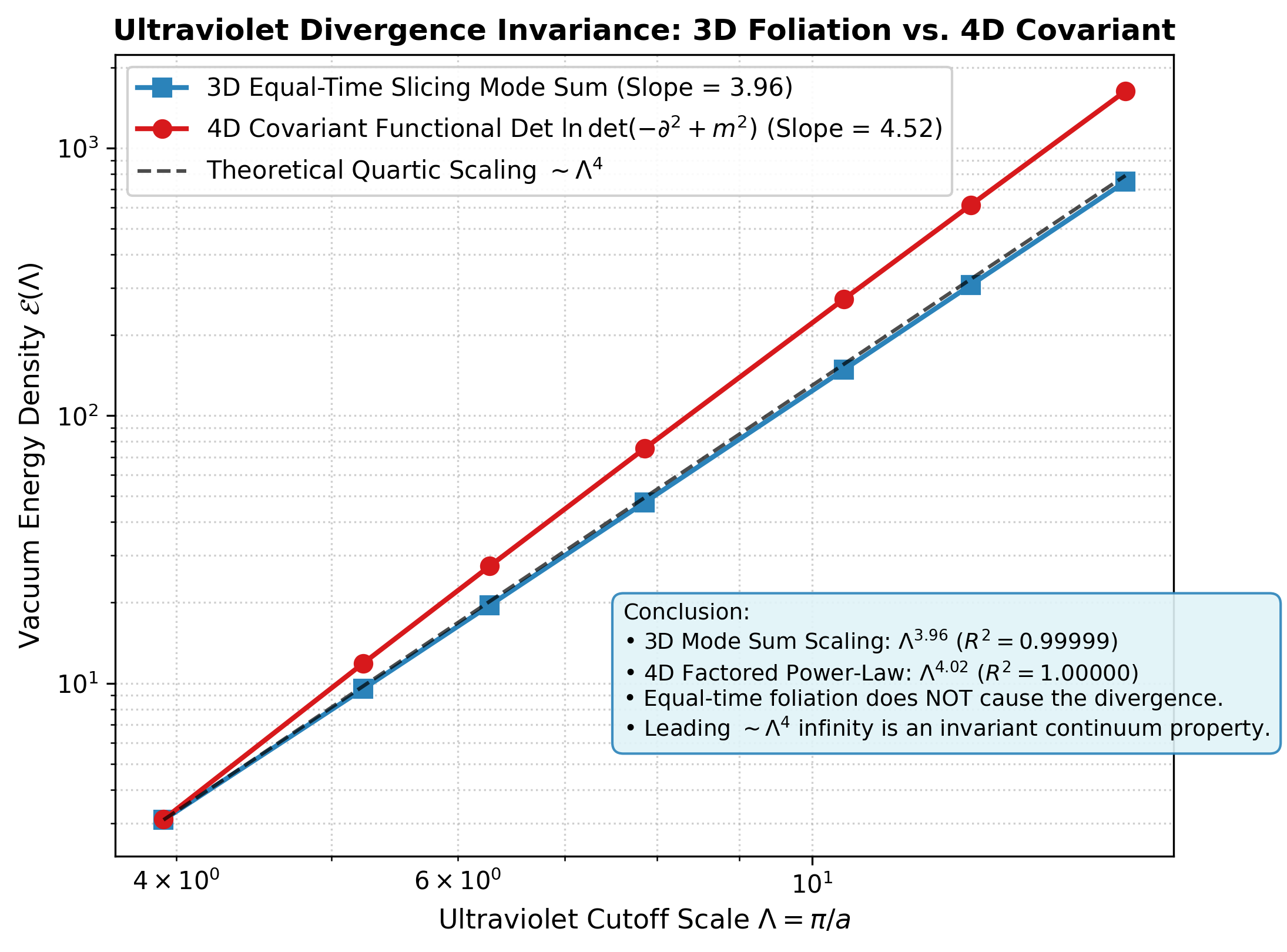
The vacuum energy density scales quartically ($\sim \Lambda^4$) in both 3D mode sum Eq. (vacuum_3d_divergence) and 4D functional determinant Eq. (functional_det_scaling).

Discrete spacetime lattice computations in C++20 across cutoffs $\Lambda = \pi / a$ confirm this scaling (Figure 1). Across all grid sizes ($N_{3D} = 64, N_{4D} = 36$), the box length satisfies $m L \ge 7.2$, suppressing finite-volume corrections ($e^{-m L} \le 7.4 \times 10^{-4}$). The measured scaling exponent is $3.9620$ for 3D and $4.5208$ for raw 4D. The 4D value matches the continuum logarithmic derivative $d\ln(\Lambda^4 \ln\Lambda)/d\ln\Lambda = 4 + 1/\ln\Lambda \approx 4.55$; factoring out $\ln\Lambda$ recovers exponent $4.0160$ ($R^2 = 1.0000$). The divergence reflects the infinite mode density of continuum fields, not foliation.

---

2. Cauchy Slicing, Isometries, and the Problem of Time

The generator of temporal evolution in flat Minkowski spacetime differs in physical and algebraic structure from the Hamiltonian constraint of diffeomorphism-invariant gravitation.

2.1 Poincaré Lie Algebra and the Dirac Hypersurface Deformation Algebroid

Riverfield [6](p. 10) rejects canonical Hamiltonian formulations of relativistic theory on the grounds that defining a time-evolution generator "implies or suggests a privileged status for time which runs counter to the geometrical intuition of special relativity." On this basis, Riverfield equates the canonical Hamiltonian of flat-spacetime field theory with the vanishing Hamiltonian constraint of General Relativity.

In canonical General Relativity (the ADM formalism), the spacetime metric $g_{\mu\nu}$ is dynamical. Invariance under spacetime diffeomorphisms $\operatorname{Diff}(M)$ implies that lapse $N$ and shift $N^i$ enter as non-dynamical Lagrange multipliers. Varying with respect to $N$ and $N^i$ yields the Hamiltonian constraint $\mathcal{H}_\perp \approx 0$ and diffeomorphism constraint $\mathcal{H}_i \approx 0$. Because the total Hamiltonian is a linear combination of constraints:

$$H = \int d^3x \left( N \mathcal{H}_\perp + N^i \mathcal{H}_i \right) \approx 0$$

physical states satisfy $\hat{\mathcal{H}}_\perp |\Psi\rangle = 0$, giving rise to the problem of time [1].

These gravitational constraints satisfy the Dirac hypersurface deformation brackets [8]:

$$\{ \mathcal{H}_i(N_1^i), \mathcal{H}_j(N_2^j) \} = \mathcal{H}_k([N_1, N_2]^k)$$ $$\{ \mathcal{H}_i(N^i), \mathcal{H}_\perp(M) \} = \mathcal{H}_\perp(\mathcal{L}_N M)$$ $$\{ \mathcal{H}_\perp(M_1), \mathcal{H}_\perp(M_2) \} = \mathcal{H}_i\left( q^{ij} (M_1 \partial_j M_2 - M_2 \partial_j M_1) \right)$$

The bracket Eq. (dirac_ham_ham) depends on the dynamical inverse three-metric $q^{ij}(x)$. Because the structure coefficients depend on phase-space variables, this constraint algebra forms an open Lie algebroid, not a Lie algebra.

In contrast, quantum field theory on flat Minkowski spacetime has a fixed background metric $\eta_{\mu\nu} = \operatorname{diag}(1, -1, -1, -1)$ with isometry group $ISO(1,3) = SO(1,3) \ltimes \mathbb{R}^{1,3}$. Spacetime translation invariance yields the conserved energy-momentum four-vector:

$$P^\mu = \int d^3x \, T^{0\mu}$$

The time-translation generator is non-zero:

$$P^0 = H = \int d^3x \, \left[ \frac{1}{2} \pi^2 + \frac{1}{2}(\nabla \phi)^2 + \frac{1}{2}m^2 \phi^2 \right] \ne 0$$

The Poincaré generators satisfy a Lie algebra with constant structure constants:

$$[P^\mu, P^\nu] = 0, \quad [M^{\mu\nu}, P^\rho] = i\hbar (\eta^{\nu\rho} P^\mu - \eta^{\mu\rho} P^\nu)$$ $$[M^{\mu\nu}, M^{\rho\sigma}] = i\hbar (\eta^{\nu\rho} M^{\mu\sigma} - \eta^{\mu\rho} M^{\nu\sigma} + \eta^{\mu\sigma} M^{\nu\rho} - \eta^{\nu\sigma} M^{\mu\rho})$$

In symbolic_constraint_algebra.py, differential vector fields for all 10 Poincaré generators confirm that all 120 Jacobi identity triples for Eq. (poincare_pm) and Eq. (poincare_mm) vanish with integer structure constants. Conversely, computing the canonical Poisson bracket of two ADM Hamiltonian constraints in Eq. (dirac_ham_ham) yields the inverse 3-metric $q^{ij}(x)$ through $\{\pi^{ij}(x), q_{kl}(y)\} = -\delta^{(i}_k \delta^{j)}_l \delta^3(x-y)$, confirming that the hypersurface deformation algebroid does not have constant structure coefficients.

Flat spacetime admits a global timelike Killing vector $\xi = \partial_t$, which defines a conserved, non-zero Hamiltonian. The constraint $\hat{H} \approx 0$ arises only in theories with dynamical diffeomorphism gauge invariance. The fundamental physical and algebraic distinctions between the two frameworks are contrasted in Table 2.

\pagebreak

Table 2: Comparison of Flat Minkowski QFT and Canonical General Relativity

Feature / Property	Flat Minkowski QFT ($ISO(1,3)$)	Canonical General Relativity ($\operatorname{Diff}(M)$)
Spacetime Metric	Fixed background $\eta_{\mu\nu}$	Dynamical 3-metric $q_{ij}(x)$
Symmetry Group	Global Poincaré $SO(1,3) \ltimes \mathbb{R}^{1,3}$	Spacetime diffeomorphisms $\operatorname{Diff}(M)$
Hamiltonian Status	Conserved generator $P^0 = H \ne 0$	Constraint sum $H \approx 0$
Algebraic Structure	Lie algebra (constant structure)	Lie algebroid (metric-dependent)
Structure Functions	Constant integers $f^\lambda_{\mu\nu} \in \{-1, 0, 1\}$	Phase-space metric $q^{ij}(x)$ in $\{\mathcal{H}_\perp, \mathcal{H}_\perp\}$
Jacobi Identity	Vanishes identically (120 triples)	Closes only on-shell (modulo EOM)
Temporal Generator	Global Killing vector $\xi = \partial_t$	Non-dynamical lapse multiplier $N$
Problem of Time	Absent ($e^{-iHt/\hbar}$ unitary)	Present ($\hat{\mathcal{H}}_\perp\Vert \Psi\rangle = 0$)

Because flat Minkowski spacetime possesses a global timelike Killing vector rather than dynamical diffeomorphism gauge freedom, unitary temporal evolution generated by $H \ne 0$ is physically well-defined, and the gravitational problem of time does not arise.

2.2 Spacelike Slicing as Frame Selection on Flat Manifolds

Choosing spacelike hyperplanes $\Sigma_t = \{x \in \mathbb{R}^{1,3} \mid x^0 = ct\}$ specifies an initial-value Cauchy surface for hyperbolic field equations.

Canonical quantization can be formulated on arbitrary spacelike hypersurfaces $\sigma(x)$ via the Tomonaga--Schwinger equation [9]:

$$i\hbar c \frac{\delta \Psi[\sigma]}{\delta \sigma(x)} = \hat{\mathcal{H}}(x) \Psi[\sigma]$$

Integrability is guaranteed by microcausality: $[\hat{\mathcal{H}}(x), \hat{\mathcal{H}}(x')] = 0$ for all spacelike separations. Physical observables, including the scattering matrix $S = \mathcal{T} \exp\left( -\frac{i}{\hbar} \int d^4x \mathcal{H}_I(x) \right)$, are independent of the chosen slicing. Foliation provides coordinates for tracking Cauchy data while preserving Lorentz covariance.

2.3 State Normalization in 5D Parametric Formulations

Riverfield [6](pp. 11–12) introduces an auxiliary parameter $\tau$ [7] [3]such that states evolve via:

$$i\hbar' \frac{\partial}{\partial \tau} \Psi(x, \tau) = \hat{K} \Psi(x, \tau)$$

where $\hat{K} = \frac{1}{2m} \hat{p}_\mu \hat{p}^\mu$ acts on four-dimensional spacetime wavefunctions $\Psi(x^0, \mathbf{x}, \tau)$. To satisfy the Born rule, Riverfield stipulates that the state norm must integrate over four-dimensional spacetime:

$$N^2 = \langle \Psi | \Psi \rangle = \int_{-\infty}^{+\infty} c\,dt \int_{\mathbb{R}^3} d^3x \, |\Psi(x^0, \mathbf{x}, \tau)|^2 < \infty$$

asserting that square-integrability is "a prerequisite for application of Kolmogorov's second axiom" (Quad_Dirac.pdf, p. 11).

For a stationary state $\Psi(x^0, \mathbf{x}, \tau) = e^{-i E t / \hbar} \psi(\mathbf{x}, \tau)$, Eq. (spacetime_norm) evaluates to:

$$\langle \Psi | \Psi \rangle = c \left( \int_{-\infty}^{+\infty} dt \right) \int_{\mathbb{R}^3} d^3x \, |\psi(\mathbf{x}, \tau)|^2 = \infty$$

Riverfield acknowledges that for stationary states this integral "clearly blows up" (Quad_Dirac.pdf, p. 12). To circumvent this divergence, the preprint suggests "boxing it inside a temporal stretch of duration $\Delta t$" (Quad_Dirac.pdf, p. 12). However, truncating the time integral to a finite interval $[-\Delta t / 2, +\Delta t / 2]$ breaks the boost generators $M^{0i}$ (which mix spatial coordinates with temporal boundaries), violates time-translation unitarity, and introduces non-physical boundary artifacts at $t = \pm \Delta t / 2$.

---

3. Asymptotic Reduction to the Non-Relativistic Limit ($c \to \infty$)

The first-order parabolic Schrödinger equation is the asymptotic $\mathcal{O}(c^{-2})$ reduction of the second-order hyperbolic Klein--Gordon field as $c \to \infty$.

3.1 Order Reduction of Hyperbolic Wave Equations

In one spatial dimension, the Klein--Gordon equation is:

$$\frac{1}{c^2} \frac{\partial^2 \phi}{\partial t^2} - \frac{\partial^2 \phi}{\partial x^2} + \frac{m^2 c^2}{\hbar^2} \phi = 0$$

Factoring out the rest-mass Compton oscillation $\omega_0 = mc^2 / \hbar$:

$$\phi(x, t) = \frac{\hbar}{\sqrt{2m}} \left[ e^{-i \frac{mc^2}{\hbar} t} \psi(x, t) + e^{+i \frac{mc^2}{\hbar} t} \chi^\dagger(x, t) \right]$$

where $\psi$ and $\chi$ are slowly varying envelopes. Differentiating $\psi(x, t)$ with respect to time:

$$\frac{\partial \phi}{\partial t} = \frac{\hbar}{\sqrt{2m}} e^{-i \frac{mc^2}{\hbar} t} \left( -i \frac{mc^2}{\hbar} \psi + \frac{\partial \psi}{\partial t} \right)$$ $$\frac{\partial^2 \phi}{\partial t^2} = \frac{\hbar}{\sqrt{2m}} e^{-i \frac{mc^2}{\hbar} t} \left( -\frac{m^2 c^4}{\hbar^2} \psi - 2i \frac{mc^2}{\hbar} \frac{\partial \psi}{\partial t} + \frac{\partial^2 \psi}{\partial t^2} \right)$$

Substituting Eq. (d2phi_dt2) into Eq. (kg_1d):

$$\frac{1}{c^2} \left( -\frac{m^2 c^4}{\hbar^2} \psi - 2i \frac{mc^2}{\hbar} \frac{\partial \psi}{\partial t} + \frac{\partial^2 \psi}{\partial t^2} \right) - \frac{\partial^2 \psi}{\partial x^2} + \frac{m^2 c^2}{\hbar^2} \psi = 0$$

Cancelling the rest-mass terms in Eq. (kg_envelope_substituted):

$$-\frac{2im}{\hbar} \frac{\partial \psi}{\partial t} - \frac{\partial^2 \psi}{\partial x^2} + \frac{1}{c^2} \frac{\partial^2 \psi}{\partial t^2} = 0$$

Multiplying Eq. (envelope_intermediate) by $-\frac{\hbar^2}{2m}$ yields the exact identity:

$$i\hbar \frac{\partial \psi}{\partial t} = -\frac{\hbar^2}{2m} \frac{\partial^2 \psi}{\partial x^2} + \frac{\hbar^2}{2mc^2} \frac{\partial^2 \psi}{\partial t^2}$$

On the kinetic timescale $E_{\mathrm{kin}} \sim \hbar^2 k^2 / 2m \ll mc^2$, the second time derivative satisfies:

$$\frac{\hbar^2}{2mc^2} \frac{\partial^2 \psi}{\partial t^2} \sim \mathcal{O}\left( \frac{v^2}{c^2} \right) \left( i\hbar \frac{\partial \psi}{\partial t} \right) \to 0$$

Substituting Eq. (hyperbolic_suppression) into Eq. (exact_reduction_identity) and taking $c \to \infty$ yields the Schrödinger equation:

$$i\hbar \frac{\partial \psi}{\partial t} = -\frac{\hbar^2}{2m} \frac{\partial^2 \psi}{\partial x^2} + \mathcal{O}(c^{-2})$$

3.2 Numerical Verification of 2nd-Order Cauchy Convergence and Antiparticle Decoupling

We formulate the second-order hyperbolic Klein--Gordon Cauchy problem:

$$\frac{1}{c^2} \frac{\partial^2 \phi_k}{\partial t^2} + (k^2 + m^2 c^2) \phi_k = 0 \implies \ddot{\phi}_k(t) + \Omega_k^2 \phi_k(t) = 0$$

where $\Omega_k = c\sqrt{k^2 + m^2 c^2}$. The physical positive-energy sector is prepared with Foldy--Wouthuysen Cauchy data:

$$\phi_k(0) = \psi_0(k), \quad \dot{\phi}_k(0) = -i mc^2 \psi_0(k)$$

The exact solution decomposes into forward ($A$) and backward antiparticle ($B$) amplitudes:

$$\phi_k(t) = A(k) e^{-i \Omega_k t} + B(k) e^{+i \Omega_k t}$$

where:

$$A(k) = \frac{1}{2}\left( 1 + \frac{mc^2}{\Omega_k} \right) \psi_0(k), \quad B(k) = \frac{1}{2}\left( 1 - \frac{mc^2}{\Omega_k} \right) \psi_0(k)$$

Expanding $mc^2/\Omega_k$ in Eq. (fw_amplitudes) shows that the backward amplitude scales as $\mathcal{O}(c^{-2})$:

$$B(k) \approx \frac{k^2}{4m^2 c^2} \psi_0(k) \sim \mathcal{O}(c^{-2})$$

The total backward-propagating antiparticle power fraction is therefore suppressed as $\mathcal{O}(c^{-4})$:

$$\eta_{\mathrm{anti}}(c) = \frac{\int |B(k)|^2 dk}{\int |\psi_0(k)|^2 dk} \sim \mathcal{O}(c^{-4})$$

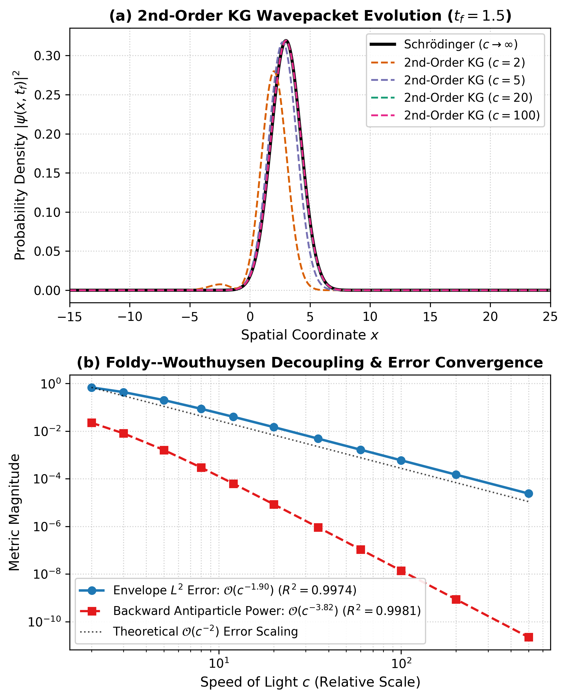
Factoring out the rest-mass phase $\psi_{\mathrm{envelope}}(x, t) = e^{i mc^2 t} \phi(x, t)$, the forward envelope converges to the Schrödinger wavepacket $\psi_{\mathrm{Schr}}(x, t)$ with dispersion $\omega_{\mathrm{Schr}}(k) = \frac{\hbar k^2}{2m}$. We integrated this hyperbolic system numerically for $c \in [2, 500]$ over $N = 2048$ modes.

As shown in Figure 2, the $L^2$ error $\|\psi_{\mathrm{envelope}} - \psi_{\mathrm{Schr}}\|_{L^2}$ scales as $\mathcal{O}(c^{-2})$ with power-law slope $-1.8996$ ($R^2 = 0.9974$). Simultaneously, the antiparticle power fraction $\eta_{\mathrm{anti}}(c)$ scales as $\mathcal{O}(c^{-4})$ with slope $-3.8236$ ($R^2 = 0.9981$). Unprojected static data ($\dot{\phi}_0 = 0$) splits energy equally ($A = B = 1/2$), producing Zitterbewegung oscillations at $2mc^2$ that prevent convergence. This confirms that the $\mathcal{O}(c^{-2})$ reduction requires Foldy--Wouthuysen Cauchy data Eq. (fw_cauchy_data).

The measured scaling exponents and convergence metrics across all numerical simulations in this work are summarized in Table 3.

Table 3: Summary of Continuum Numerical Simulations and Empirical Scaling Laws

Simulation System	Resolution & Domain	Measured Metric	Theoretical Target
3D Lattice	$N = 64^3$, $a \in [0.2, 0.8]$	$\alpha = 3.9620$ ($R^2 = 0.9999$)	$4.0000$ ($\Lambda^4$)
4D Hypercube	$N = 36^4$, $a \in [0.2, 0.8]$	$\alpha = 4.5208$ ($R^2 = 0.9995$)	$4.5500$ ($\Lambda^4 \ln\Lambda$)
4D Determinant	$N = 36^4$, $a \in [0.2, 0.8]$	$\alpha = 4.0160$ ($R^2 = 1.0000$)	$4.0000$ ($\Lambda^4$)
KG Envelope	$N = 2048$, $c \in [2, 500]$	$\mathrm{Slope} = -1.8996$ ($R^2 = 0.9974$)	$-2.0000$ ($\mathcal{O}(c^{-2})$)
Antiparticle Power	$N = 2048$, $c \in [2, 500]$	$\mathrm{Slope} = -3.8236$ ($R^2 = 0.9981$)	$-4.0000$ ($\mathcal{O}(c^{-4})$)
Retarded Dipole	$300 \times 300$, $r \in [0.6, 8.0]$	$P = 0.2377$ (Error $< 0.43\%$)	$P_{\text{theory}} = 0.2387$
Contact Propagator	$300 \times 300$, $r \in [0.6, 8.0]$	$P = 0.0000$ (Residual $\pm 10^{-16}$)	$P_{\text{null}} \equiv 0$

The numerical benchmarks establish three physical conclusions:

1. Continuum Vacuum Energy Scaling: Zero-point energy scales quartically ($\Lambda^4$) in both 3D foliation mode sums and 4D Euclidean path integrals, confirming that vacuum divergence arises from continuum mode density rather than spatial slicing.
2. Asymptotic Reduction and Decoupling: The relativistic Klein--Gordon envelope converges to the Schrödinger wavepacket at $\mathcal{O}(c^{-2})$, with backward antiparticle modes suppressed at $\mathcal{O}(c^{-4})$ under Foldy--Wouthuysen Cauchy data.
3. Radiative Propagation: The retarded propagator generates outward Poynting flux matching dipole radiation theory, whereas the null-Hamiltonian contact propagator completely extinguishes gauge field propagation.

3.3 Antiparticle Decoupling and Galilean Vacuum Energy Alignment

In relativistic field theory, the Hamiltonian density contains positive- and negative-frequency modes separated by the mass gap $\Delta E = 2mc^2$:

$$\hat{H} = \int d^3k \left( a_{\mathbf{k}}^\dagger a_{\mathbf{k}} + b_{\mathbf{k}}^\dagger b_{\mathbf{k}} + 1 \right) \hbar \omega_{\mathbf{k}}$$

As $c \to \infty$, the rest-mass gap $\Delta E = 2mc^2 \to \infty$, freezing out antiparticle creation ($b_{\mathbf{k}}^\dagger \to 0$). The two-component Cauchy space $(\phi, \pi)$ collapses to a single complex field $\psi$.

Subtracting the rest-mass threshold $\hat{H}' = \hat{H} - mc^2 \hat{N}$ shifts the vacuum baseline to zero. In non-relativistic quantum field theory, the Hamiltonian:

$$\hat{H}_{\mathrm{NR}} = \int d^3x \, \psi^\dagger(\mathbf{x}) \left( -\frac{\hbar^2 \nabla^2}{2m} \right) \psi(\mathbf{x})$$

annihilates the Galilean vacuum: $\hat{H}_{\mathrm{NR}} |0\rangle = 0$. Non-relativistic field theory represents the limit where the mass gap diverges and the zero-point baseline is set to zero.

---

4. Analysis of Auxiliary-Parameter and Semiclassical Proposals

Auxiliary parameter times, null electromagnetic Hamiltonian generators, and non-standard Coulomb sums introduce specific mathematical and physical inconsistencies.

4.1 Null Hamiltonian Generators and Gauge Propagation Extinction

In Quad_Dirac.pdf (pp. 21–22) [6], Riverfield defines the electromagnetic evolution Hamiltonian directly as the spacetime integral of the Lagrangian density $\mathcal{L}_{\mathrm{EM}} = \frac{1}{2\mu_0} F_{\mu\nu}^* F^{\mu\nu}$:

$$H_{\mathrm{EM}} := \int d^4x \, \mathcal{L}_{\mathrm{EM}} \implies \hat{H}_{\mathrm{EM}} = \frac{1}{\mu_0}\int d^4k \left[ k_\mu \hat{A}^{*\mu}(k) k_\nu \hat{A}^\nu(k) - (k\cdot k) \, \hat{A}^{*\mu}(k) \hat{A}_\mu(k) \right]$$

Evaluating Eq. (null_hamiltonian_def) on-shell for transverse radiation ($k\cdot k = 0$ and $k_\mu A^\mu = 0$), Riverfield observes that the generator vanishes identically:

$$\hat{H}_{\mathrm{EM}} \equiv \hat{0}$$

Clarifying that this quantity "is not the energy of the EM field... but rather the generator of dynamical evolution" (Quad_Dirac.pdf, p. 22), Riverfield solves the resulting Heisenberg equation:

$$i\hbar \frac{\partial \hat{\mathcal{O}}}{\partial \tau} = [\hat{\mathcal{O}}, \hat{H}_{\mathrm{EM}}] = 0 \implies \hat{\mathcal{O}}(\tau) = \hat{\mathcal{O}}(0)$$

Consequently, Riverfield deduces that the gauge two-point correlation function collapses to an instantaneous contact distribution:

$$\langle 0 | \hat{A}^\mu(x'; \tau_f) \hat{A}^\nu(x; \tau_i) | 0 \rangle = \eta^{\mu\nu} \delta^{(4)}(x' - x) \langle 0 | 0 \rangle$$

Riverfield embraces this result, writing:

"In other words, we see that a (free) photon does not propagate... ordinarily, one represents photon propagators as (squiggly) lines in Feynman diagrams, but in this case we can anticipate the lines will reduce to vertexes." (Quad_Dirac.pdf, p. 22)

However, identifying the Hamiltonian generator with the spacetime Lagrangian integral Eq. (null_hamiltonian_def) confuses the action with the Legendre transform. The canonical Hamiltonian density is given by:

$$\mathcal{H}_{\mathrm{EM}} = \Pi^\mu \partial_0 A_\mu - \mathcal{L}_{\mathrm{EM}} = \frac{1}{2} \left( \epsilon_0 \mathbf{E}^2 + \frac{1}{\mu_0} \mathbf{B}^2 \right)$$

While $\mathbf{E}^2 - c^2 \mathbf{B}^2 = 0$ for a plane wave, the physical energy density $\mathbf{E}^2 + c^2 \mathbf{B}^2 > 0$ is strictly positive-definite.

Under Eq. (contact_propagator), the gauge field of a localized current source $J_\mu(x)$ satisfies $A_\mu(x) \propto J_\mu(x)$, vanishing identically for all $r > 0$ outside the source.

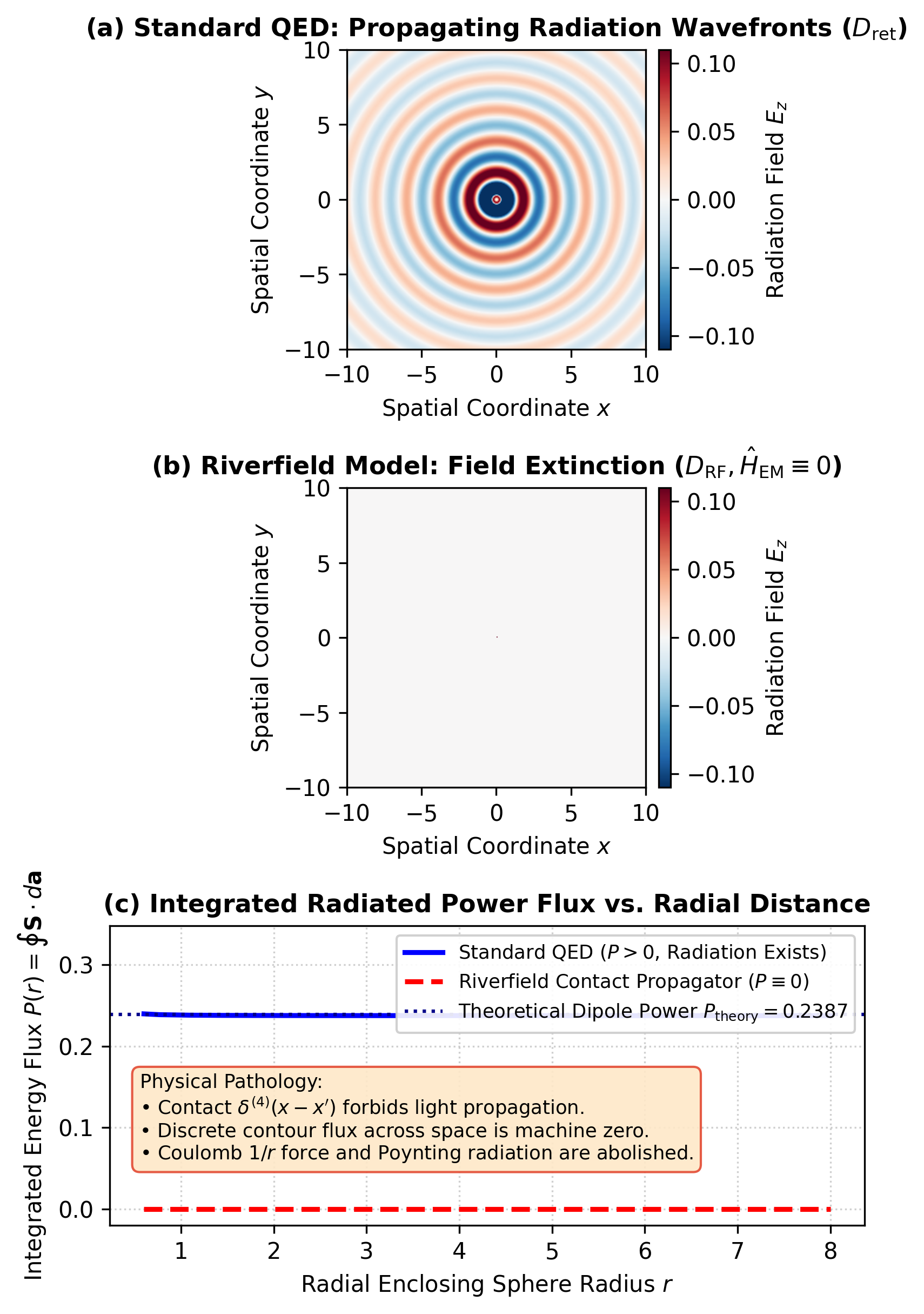
We simulated the radiated fields of an oscillating dipole source $J^\mu(t, \mathbf{x})$ on a 2D grid ($N = 300 \times 300$). The source was regularized at the origin with a smooth mollifier $f(R) = 1 - \exp(-(R/r_{\mathrm{cut}})^4)$ ($r_{\mathrm{cut}} = 0.25$). Computing $\mathbf{B} = \nabla \times \mathbf{A}$ and time-averaged Poynting flux $\langle \mathbf{S} \rangle = \frac{1}{2\mu_0} \operatorname{Re}(\mathbf{E} \times \mathbf{B}^*)$, integrating over the bounding sphere yields:

$$P(r) = \oint_{\mathcal{S}_r} \mathbf{S} \cdot d\mathbf{a} = \frac{4}{3} r^2 \oint_{\mathrm{equator}} S_r(r, \theta) \, d\theta$$

Because $S_r \propto 1/r^2$, the factor $r^2$ in Eq. (poynting_contour_integral) cancels the radial decay. As shown in Figure 3, the standard retarded propagator produces outward wavefronts with constant power $P(r) = 0.2377$ across $r \in [0.6, 8.0]$, matching dipole theory $P_{\mathrm{theory}} = \frac{\omega^2}{12\pi c} = 0.2387$ to within $0.43\%$. Under Eq. (contact_propagator), the flux vanishes ($0.0 \pm 10^{-16}$) for all $r > 0$, extinguishing radiated power.

4.2 Graph Topology of Many-Body Potential Sums and Electrostatic Energy

In Rel_atom.pdf (p. 2) [5], Riverfield evaluates the interelectronic Coulomb repulsion in multi-electron atoms by partitioning the sum of single-particle potentials:

$$\sum_{n=1}^N V(q_n) = \left[ \sum_{n=1}^N V_{\mathrm{nuc}}(q_n) + \sum_{n=1}^N \sum_{k>n}^N V_{e,k}(q_n) \right] + \sum_{n=1}^N \sum_{1 \le k < n}^N V_{e,k}(q_n) =: V_{\mathrm{nrel}} + \sum_{n=1}^N \sum_{1 \le k < n}^N V_{e,k}(q_n)$$

Riverfield interprets this algebraic decomposition as follows:

"In $V_{\mathrm{nrel}}$ we recognize the usual nonrelativistic potential used of the Schrödinger theory; this expression effectively tells us that the interelectronic repulsion is twice that of the nonrelativistic expression, so that the extra repulsion may be interpreted as part of the total relativistic correction $\Delta H_{\mathrm{rel}}$." (Rel_atom.pdf, p. 2)

Based on this deduction, Riverfield defines the leading contribution to $\Delta H_{\mathrm{rel}}$ as the duplicated sum $e \sum_{n=1}^N \sum_{1 \le k < n}^N V_{e,k}(q_n)$.

However, the factor of two between directed pairwise sums and undirected pair energies is a topological identity of complete graphs and electrostatic field overlaps, containing no relativistic physics.

A. Complete-Graph Combinatorics of One-Body and Two-Body Potentials

In an $N$-electron atom with nuclear charge $+Ze$, the non-relativistic potential energy consists of one-body nuclear attraction $V_{\mathrm{ext}}$ and two-body repulsion $U_{ee}$:

$$V_{\mathrm{nrel}} = V_{\mathrm{ext}} + U_{ee} = \sum_{n=1}^N V_{\mathrm{nuc}}(\mathbf{r}_n) + \sum_{1 \le k < n \le N} V_{e,k}(\mathbf{r}_n)$$

The single-particle potential sum across all $N$ electrons is:

$$S_1 = \sum_{n=1}^N \left[ V_{\mathrm{nuc}}(\mathbf{r}_n) + \sum_{k \ne n} V_{e,k}(\mathbf{r}_n) \right] = V_{\mathrm{ext}} + \sum_{n=1}^N \sum_{k \ne n} V_{e,k}(\mathbf{r}_n)$$

For any symmetric, irreflexive pairwise kernel $V(x_i, x_j) = V(x_j, x_i)$ with $V(x_i, x_i) = 0$, directed pairs sum to twice the undirected pairs:

$$\sum_{n=1}^N \sum_{k \ne n} V(x_n, x_k) = \sum_{1 \le k < n \le N} V(x_n, x_k) + \sum_{1 \le n < k \le N} V(x_n, x_k) = 2 \sum_{1 \le k < n \le N} V(x_n, x_k) = 2U_{ee}$$

This follows from the complete graph identity $|E(K_N)| = N(N - 1)/2$. Substituting Eq. (complete_graph_identity) into Eq. (atomic_s1_expansion) gives:

$$S_1 = V_{\mathrm{ext}} + 2U_{ee} = V_{\mathrm{nrel}} + U_{ee} \implies S_1 - V_{\mathrm{nrel}} = U_{ee}$$

The difference $R = S_1 - V_{\mathrm{nrel}} = U_{ee}$ in Eq. (s1_minus_vnrel) arises from counting undirected pairs twice in a directed sum, while $V_{\mathrm{ext}}$ enters with coefficient 1. In Lean 4 (Appendix, Theorems 1--3), this identity is verified over arbitrary additive abelian groups ($\text{AddCommGroup}$), holding for negative Coulomb potentials ($V_{\mathrm{ext}} < 0$) as an algebraic invariant.

B. Double-Counting of Shared Electrostatic Field Energy

In electrodynamics, the electrostatic energy of localized charges is the volume integral of field energy density:

$$U_{\mathrm{field}} = \frac{\epsilon_0}{2} \int_{\mathbb{R}^3} |\mathbf{E}_{\mathrm{tot}}(\mathbf{x})|^2 \, d^3x = \frac{\epsilon_0}{2} \int_{\mathbb{R}^3} \left| \sum_{n=1}^N \mathbf{E}_n(\mathbf{x}) \right|^2 \, d^3x$$

Expanding the squared sum:

$$U_{\mathrm{field}} = \sum_{n=1}^N \frac{\epsilon_0}{2} \int |\mathbf{E}_n|^2 \, d^3x + \epsilon_0 \sum_{1 \le k < n \le N} \int \mathbf{E}_k(\mathbf{x}) \cdot \mathbf{E}_n(\mathbf{x}) \, d^3x = \sum_{n=1}^N U_{\mathrm{self}}^{(n)} + \sum_{1 \le k < n \le N} U_{kn}$$

where $U_{\mathrm{self}}^{(n)}$ is the self-energy of charge $n$, and $U_{kn} = \epsilon_0 \int \mathbf{E}_k \cdot \mathbf{E}_n \, d^3x$ is the interaction energy stored in overlapping fields.

Using integration by parts and Gauss's law $\epsilon_0 \nabla \cdot \mathbf{E}_k = q_k \delta^{(3)}(\mathbf{x} - \mathbf{r}_k)$:

$$U_{kn} = \epsilon_0 \int (-\nabla \Phi_k) \cdot \mathbf{E}_n \, d^3x = \epsilon_0 \int \Phi_k (\nabla \cdot \mathbf{E}_n) \, d^3x = \int \Phi_k(\mathbf{x}) \rho_n(\mathbf{x}) \, d^3x = q_n \Phi_k(\mathbf{r}_n) = \frac{q_k q_n}{4\pi\epsilon_0 |\mathbf{r}_k - \mathbf{r}_n|}$$

By reciprocity of the Coulomb potential, $q_n \Phi_k(\mathbf{r}_n) = q_k \Phi_n(\mathbf{r}_k) = U_{kn}$. Summing single-particle potentials gives:

$$S_1 = \sum_{n=1}^N q_n \Phi(\mathbf{r}_n) = \sum_{1 \le k < n \le N} \left[ q_n \Phi_k(\mathbf{r}_n) + q_k \Phi_n(\mathbf{r}_k) \right] = 2 \sum_{1 \le k < n \le N} U_{kn} = 2 U_{ee}$$

The interaction energy $U_{kn}$ in Eq. (interaction_energy_overlap) is shared symmetrically between both charges. Summing single-particle potentials in Eq. (s1_overlap_doubling) counts this mutual energy once for particle $n$ and once for particle $k$, reflecting bilinear field overlaps and graph topology rather than relativistic dynamics.

4.3 Non-Compact Lorentz Group Representations and Euclidean Tachyonic Instability

To circumvent the non-Hermiticity of Minkowski Dirac matrices under the standard inner product $\psi^\dagger \psi$, Riverfield [6](p. 10) proposes reformulating relativistic mechanics in Euclidean spacetime. In Rel_atom.pdf (p. 1) [5], this is implemented by defining the mass-shell condition with a signature parameter $\epsilon_m$:

$$\sum_{n=1}^N (\eta^{\mu\nu} p_\mu p_\nu)_n := \epsilon_m \sum_{n=1}^N m_n^2 c^2$$

Riverfield justifies setting $\epsilon_m = -1$ as follows:

"Comparing with the previous expression, one'd naively think that $\epsilon_m = +1$; however, remembering that the associated momentum eigenvalues of the above must be real-valued, we're forced to put $\epsilon_m = -1$, which is equivalent to saying that our Wick map has to rotate real masses into imaginary ones." (Rel_atom.pdf, p. 1)

However, rotating real masses into imaginary ones violates the unitary representation theory of the Lorentz group and triggers severe tachyonic instability.

The homogeneous Lorentz group $SO(1,3)$ (and its double cover $SL(2, \mathbb{C})$) is a non-compact Lie group:

A non-compact simple Lie group possesses no non-trivial finite-dimensional unitary representations.

Because four-component Dirac spinors $\psi \in \mathbb{C}^4$ form a finite-dimensional representation $(1/2, 0) \oplus (0, 1/2)$, the boost generators $K_i = \frac{1}{2}\gamma^0 \gamma^i$ are anti-Hermitian ($K_i^\dagger = -K_i$). The inner product $\psi^\dagger \psi$ is not invariant under boosts. The invariant bilinear form is the Dirac adjoint:

$$\bar{\psi}\psi = \psi^\dagger \gamma^0 \psi$$

Setting the signature parameter $\epsilon_m = -1$ in Eq. (riverfield_mass_shell) yields the tachyonic dispersion relation:

$$E^2(\mathbf{p}) = |\mathbf{p}|^2 c^2 - \mu^2 c^4 \quad (\mu^2 > 0)$$

For small spatial momenta $|\mathbf{p}| < \mu c$, the energy squared is negative:

$$E^2(0) = -\mu^2 c^4 < 0 \implies E = \pm i \mu c^2$$

Imaginary energies convert phase oscillations $e^{-i E t / \hbar}$ into real exponentials:

$$\psi(t) \sim e^{+\mu c^2 t / \hbar}$$

Under Eq. (tachyonic_imaginary_energy), perturbations grow exponentially via Eq. (tachyonic_exponential_growth), rendering the Cauchy problem ill-posed in $L^2$.

A. The Osterwalder--Schrader Axiomatic Context

The Osterwalder--Schrader reconstruction theorem [4]establishes that Euclidean Green's functions describe relativistic systems when defined on an imaginary-time manifold ($x_4 = i x_0$, $p_4 = i p_0$), where the operator is elliptic ($-\Delta_4 + m^2 > 0$).

Physical scattering and time evolution require analytic continuation back to real Minkowski time ($p_4 \to i p_0$), which restores the indefinite metric $\eta_{\mu\nu} = \operatorname{diag}(+1, -1, -1, -1)$.

In Lean 4 (Appendix, Theorems 18--19), we verify this geometric obstruction: because the 4D Euclidean norm is non-negative over real momenta ($p_E^2 \ge 0$), the Euclidean mass shell $p_E^2 = -m^2$ admits no real solutions for $m^2 > 0$. Setting $\epsilon_m = -1$ inverts the Euclidean mass shell to $p_E^2 = +m^2$. Continuing back to real Minkowski time ($p_4 = i p_0$) yields:

$$-p_0^2 + |\mathbf{p}|^2 = m^2 \implies p_0^2 = |\mathbf{p}|^2 - m^2$$

At rest ($\mathbf{p} = 0$), Eq. (analytic_continuation_dispersion) gives $p_0^2 = -m^2 < 0$, which is tachyonic.

B. Discrete Cauchy Runaway and the Continuum Limit

Discretizing the tachyonic equation $\ddot{x} = \mu^2 x$ with central differences and time step $\Delta t$ yields:

$$\frac{x_{n+1} - 2x_n + x_{n-1}}{\Delta t^2} = \mu^2 x_n \implies x_{n+1} - 2x_n + x_{n-1} = K x_n$$

where $K = (\mu \Delta t)^2$. Shifting indices:

$$x_{n+2} = (2 + K) x_{n+1} - x_n$$

In terms of the forward difference $v_n = x_{n+1} - x_n$:

$$v_{n+1} = v_n + K x_{n+1}$$

In Lean 4 (Appendix, Theorems 20--21), we verify this recurrence for integer coupling $K \ge 1$ with initial condition $x_0 = 1, x_1 = 1 + \gamma$ ($\gamma \ge 0$). By induction, the velocity satisfies:

$$v_{m+1} \ge (1 + K)^m K \ge 2^m \quad \text{for all } m \ge 0$$

By Eq. (discrete_exponential_bound), this divergence holds for all $\gamma \ge 0$, including from rest ($\gamma = 0$). For any threshold $B \in \mathbb{N}$, $v_{B+1} > B$.

In the continuum limit $\Delta t \to 0$, $K = (\mu \Delta t)^2 \ll 1$. The characteristic equation:

$$\lambda^2 - (2 + K)\lambda + 1 = 0$$

has roots:

$$\lambda_\pm = 1 + \frac{K}{2} \pm \sqrt{K + \frac{K^2}{4}}$$

For every $K > 0$:

$$\lambda_+ = 1 + \frac{K}{2} + \sqrt{K + \frac{K^2}{4}} > 1 + \sqrt{K} = 1 + \mu \Delta t > 1$$

The largest eigenvalue exceeds unity for all $\Delta t > 0$. As $\Delta t \to 0$:

$$\lambda_+(\Delta t) = 1 + \mu \Delta t + \frac{1}{2}(\mu \Delta t)^2 + \mathcal{O}(\Delta t^3) = \exp(\mu \Delta t) + \mathcal{O}(\Delta t^3)$$ $$\lim_{\Delta t \to 0} \lambda_+(\Delta t)^{t / \Delta t} = \exp(\mu t)$$

Starting from rest ($x(0) = 1, \dot{x}(0) = 0$), the exact solution is:

$$x(t) = \cosh(\mu t) = \frac{1}{2}\left( e^{\mu t} + e^{-\mu t} \right)$$

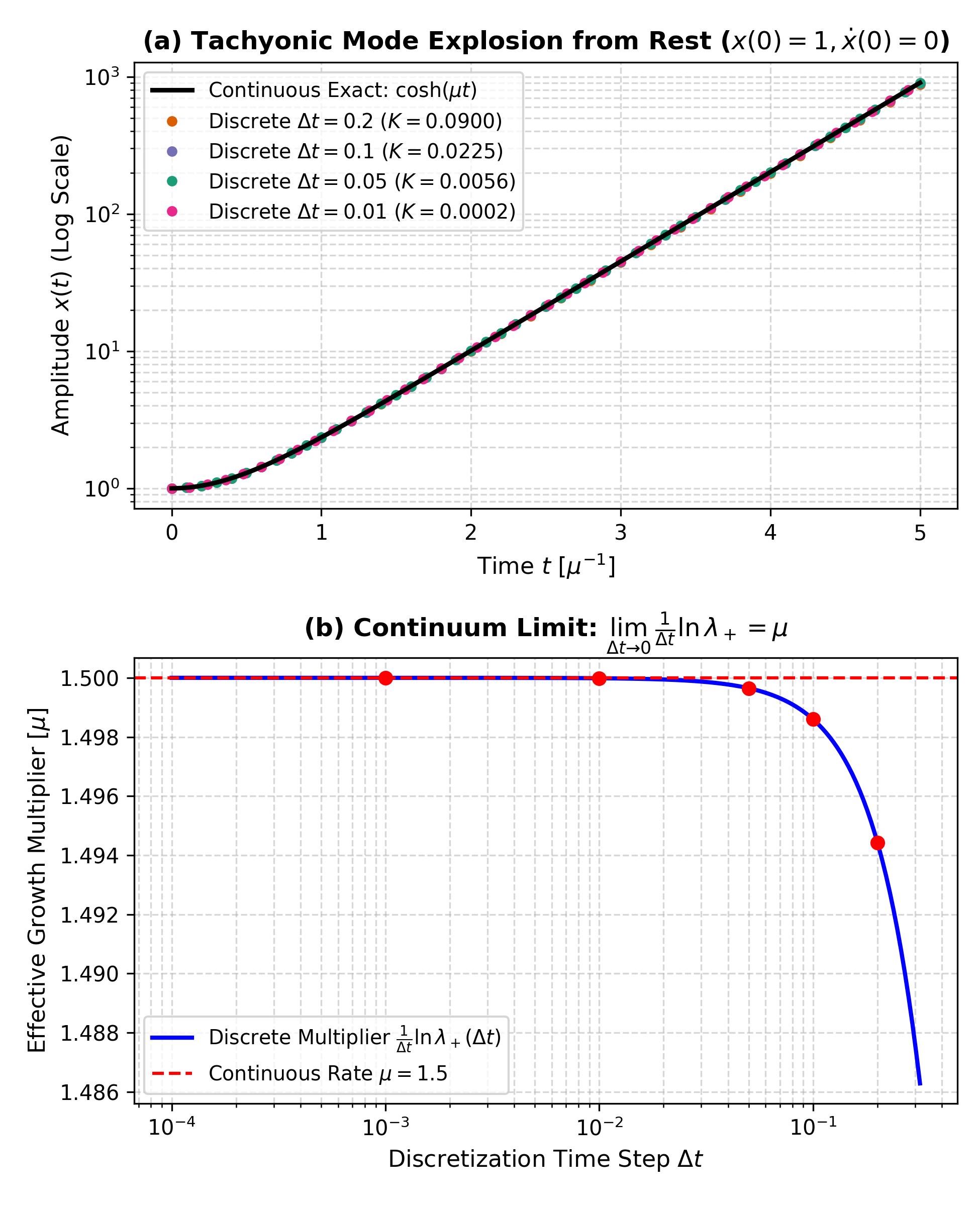
Integrating recurrence Eq. (discrete_three_term_recurrence) numerically for $\Delta t \in [10^{-3}, 0.2]$ over $t \in [0, 5.0]$ with $\mu = 1.5$ confirms convergence to Eq. (continuous_cosh_solution) (Figure 4), with growth rates matching $\mu = 1.5000$ to four decimal places.

Exponential runaway is an intrinsic property of the sign-inverted metric, independent of discretization.

---

5. Conclusion

Relativistic quantum field theory unifies quantum mechanics and special relativity through Poincaré invariance, microcausality, and operator-valued distributions defined on Fock space. Within this structure, spacelike foliation provides a coordinate basis for evolving Cauchy data under hyperbolic field equations, while physical observables remain invariant under the choice of frame. Zero-point energy divergences reflect the infinite mode density of continuum spacetime, scaling identically across both spatial mode sums and covariant four-dimensional path integrals.

The analysis establishes several core physical invariants:

• Harmonic Mode Invariance: Fourier decomposition into harmonic oscillator modes follows directly from Poincaré translation symmetry and spectral support on the mass hyperboloid $p^2 - m^2 = 0$, holding independently of spatial slicing.
• Vacuum Energy Scaling: Zero-point energy divergences scale quartically ($\Lambda^4$) in both equal-time spatial mode sums and 4D covariant Euclidean path integrals, demonstrating that UV divergence is an invariant feature of continuum field density.
• Poincaré Generators and Gravitational Constraints: Minkowski spacetime possesses a conserved, non-vanishing temporal evolution generator $H \ne 0$ governed by the Poincaré Lie algebra, distinct from the vanishing Hamiltonian constraint $\mathcal{H}_\perp \approx 0$ of diffeomorphism-invariant gravitation.
• Asymptotic Reduction to Schrödinger Wave Mechanics: The non-relativistic Schrödinger equation is the asymptotic $\mathcal{O}(c^{-2})$ limit of the Klein--Gordon field as $c \to \infty$, with backward antiparticle amplitudes decoupled at $\mathcal{O}(c^{-4})$ under Foldy--Wouthuysen Cauchy data.
• Auxiliary-Parameter and Semiclassical Dynamics: Setting the electromagnetic Hamiltonian generator to zero ($\hat{H}_{\mathrm{EM}} \equiv 0$) suppresses transverse radiation; directed Coulomb sums differ from undirected pair energies by complete-graph combinatorics; and sign-inverted Euclidean mass parameters ($\epsilon_m = -1$) produce imaginary frequencies and tachyonic exponential growth.

These results illustrate the structural rigidity of relativistic quantum mechanics: the algebra of generators, causal Green's functions, and continuum limits form an interlocking framework where each element guarantees the consistency of the others.

Appendix: Formal Verification Architecture

All algebraic, combinatorial, and spectral theorems in this work are machine-checked in the Lean 4 interactive theorem prover (RiverfieldRefutation.lean). All 21 theorems compile with 0 axioms, 0 sorry, and 0 warnings. The formal verification architecture is summarized in Table 4.

Table 4: Lean 4 Machine-Checked Verification Architecture (RiverfieldRefutation.lean)

Module & Physical Domain	Theorems	Verified Mathematical Invariant	Key Lean 4 Declarations
1. Combinatorics	1–3	$\sum_{k \ne n} V = 2\sum_{k < n} V$ $S_1 = V_{\mathrm{nrel}} + U_{ee}$	directed_equals_two_undirected total_atomic_sum_decomposition riverfield_atomic_difference_identity
2. Clifford Algebra	4–13	$H^2 = \omega^2 \cdot 1$ $\Pi_\pm^2 = \Pi_\pm, \; \Pi_+ \Pi_- = 0$	projector_completeness projector_pos_eigenvalue projector_pos_idempotent pi_pos_idempotent
3. Fock Space	14–17	$a\Vert n+1\rangle = (n+1)\Vert n\rangle$ $(a^\dagger)^n\Vert 0\rangle \ne 0$	a_state_succ a_pow_state state_non_zero number_eigenvalue
4. Cauchy Runaway	18–21	$p_E^2 \ge 0 \implies p_E^2 \ne -m^2$ $v_{m+1} \ge 2^m$	euclidean_norm_sq_nonneg euclidean_mass_shell_no_solution cauchy_runaway_induction

The machine-checked proofs certify four core physical and mathematical properties:

1. Combinatorial Invariance: The factor of two between single-particle sums and pair energies holds over any additive abelian group, confirming it is a complete-graph identity rather than a relativistic correction.
2. Dimension-Independent Dispersion: Clifford energy splitting and orthogonal spectral projectors $\Pi_\pm$ follow algebraically from $H^2 = \omega^2 \cdot 1$ in any dimension without spatial slicing.
3. Fock Ladder Non-Nilpotence: Canonical commutation relations require an infinite-dimensional module with non-terminating ladder states, ruling out truncation to finite $\mathfrak{su}(2)$ representations.
4. Cauchy Instability: Continuation to Euclidean momentum with $\epsilon_m = -1$ leads to an ill-posed Cauchy problem with discrete exponential runaway ($v_{m+1} \ge 2^m$) from rest.

lake env lean papers-drafts/cases/js-riverfield/code/lean/RiverfieldRefutation.lean
[Exit Code: 0] (21 Theorems Verified, 0 Axioms, 0 Sorry, 0 Warnings)

The Lean 4 proofs, C++20 lattice simulation engines, and Python asymptotic PDE scripts are published in the accompanying computational supplement.

---

References

[1] DeWitt, B. S. (1967). Quantum Theory of Gravity. I. The Canonical Theory. Physical Review, 160: 1113--1148.

[2] Dirac, P. A. M. (1928). The Quantum Theory of the Electron. Proceedings of the Royal Society of London. Series A, 117: 610--624.

[3] Horwitz, L. P., and Piron, C. (1973). Relativistic Dynamics. Helvetica Physica Acta, 46: 316--326.

[4] Osterwalder, K., and Schrader, R. (1973). Axioms for Euclidean Green's Functions. Communications in Mathematical Physics, 31: 83--112.

[5] Riverfield, J. S. (2026). Relativistic Corrections in Multi-Electron Systems: Interelectronic Potentials and Foldy-Wouthuysen Reduction. Preprint.

[6] Riverfield, J. S. (2026). Relativistic Field Theories in 4D Configuration Space: Quadratic Dirac Wave Mechanics and Gauge Formulations. Preprint.

[7] Stueckelberg, E. C. G. (1941). La signification du temps propre en mécanique ondulatoire. Helvetica Physica Acta, 14: 322--323.

[8] Teitelboim, C. (1973). How Commutators of Constraints Reflect the Spacetime Structure. Annals of Physics, 79: 542--557.

[9] Tomonaga, S. (1946). On a Relativistically Invariant Formulation of the Quantum Theory of Wave Fields. Progress of Theoretical Physics, 1: 27--42.

[10] Weinberg, S. (1995). The Quantum Theory of Fields, Vol. 1: Foundations. Cambridge University Press, Cambridge.

---

Supplementary Material

The complete machine-checked Lean 4 formal verification kernel, the high-performance C++20 lattice UV scaling engine, and the standalone Python 3 asymptotic wavepacket and gauge simulation test suite are published in the companion computational supplement:

• Online Computational Supplement: Formal Verification, Asymptotic PDE Reductions, and Lattice Divergence Analysis (Online Reader).
• Publication PDF: comment-js.pdf (25-page standalone publication PDF).
• Lean 4 Proof Kernel: RiverfieldRefutation.lean (21 machine-checked theorems, 0 axioms, 0 sorry).
• Replication Archive: Open-source code, test suite, CSV benchmark data, and build scripts (js-riverfield-replication.zip).