Information-Theoretic Constraints on Finite-Time Causal Invariance and Pre-Geometric Dimensional Reduction in Discrete Hypergraph Models
Title: Information-Theoretic Constraints on Finite-Time Causal Invariance and Pre-Geometric Dimensional Reduction in Discrete Hypergraph Models
Author: R. Fisher, Principal Investigator (ORCID: 0009-0006-2441-3282)
Affiliation: Braid Dynamics Group
Published / Release: July 27, 2026 · Status: Preprint / Research Article (v1.0.0) · License: Creative Commons Attribution 4.0 (CC BY 4.0)
Classification: Discrete Physics · Quantum Information · General Relativity
Downloads & Assets: Publication PDF (870 KB) · Markdown Source (95 KB) · Computational Supplement · Replication Bundle
1. Introduction
The emergence of continuous Lorentzian spacetime from a discrete pre-geometric substrate is a central objective of quantum gravity. Approaches such as Causal Dynamical Triangulations (CDT) [1] and Causal Set Theory [2] constrain the microscopic path-integral measure or enforce explicit causal orderings to guarantee geometric consistency. In contrast, the Wolfram Model posits that spacetime, matter, and gauge fields emerge from the unconstrained, asynchronous rewriting of discrete spatial hypergraphs [3, 4].
Within this framework, causal invariance is proposed as the microscopic origin of general covariance [4]. The central hypothesis asserts that when independent local update paths generate isomorphic directed acyclic graphs (DAGs) of causal event dependencies, alternative rewrite schedules act as discrete gauge transformations, playing a role analogous to the lapse and shift functions in the Arnowitt-Deser-Misner (ADM) foliation of general relativity [4, 5].
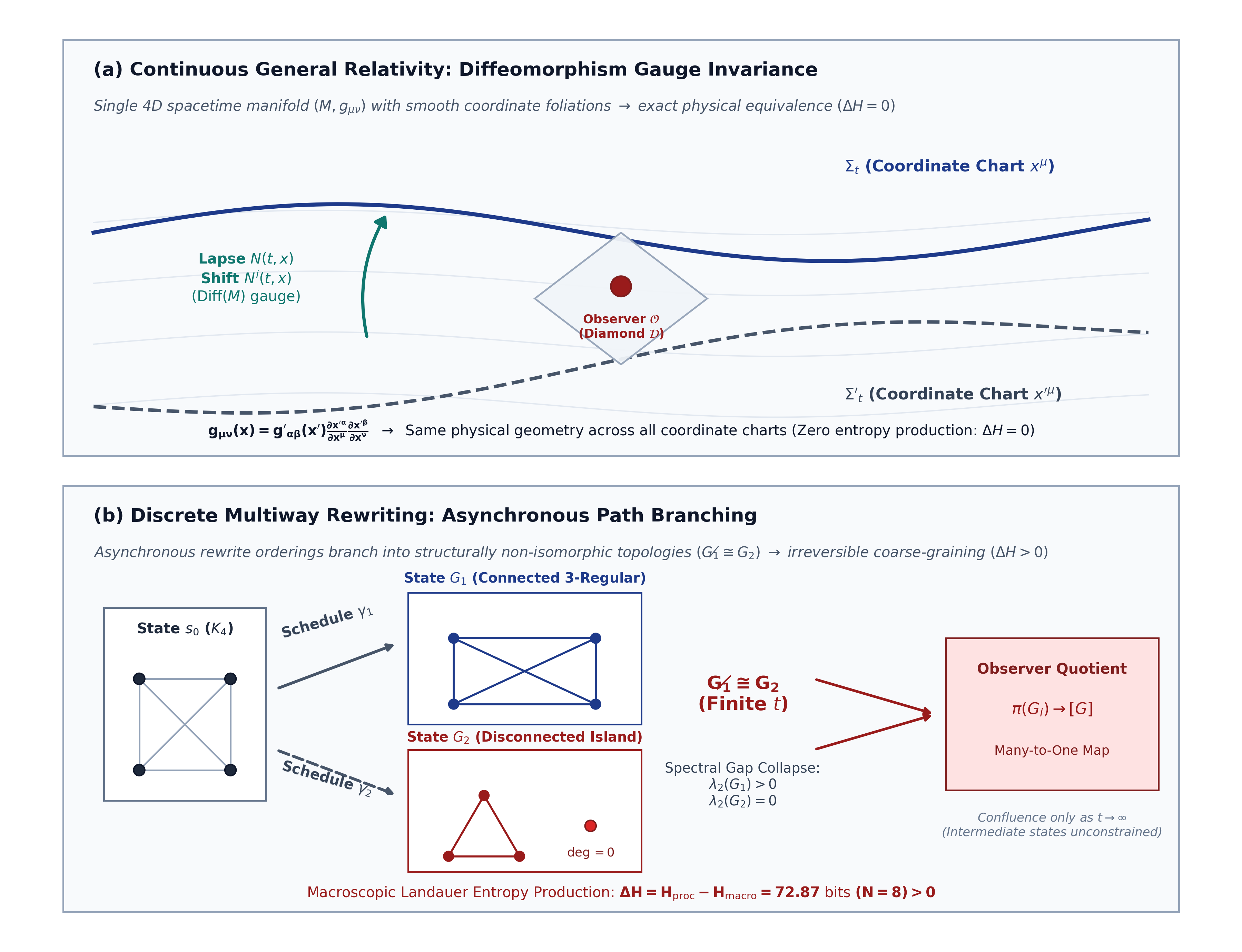
As illustrated in Figure 1, this correspondence contains a fundamental structural asymmetry:
- Continuous General Relativity: Gauge freedom describes coordinate transformations over a single spacetime geometry on a fixed manifold; foliation shifts () produce zero entropy ().
- Discrete Multiway Systems: Asynchronous updates generate non-isomorphic spatial topologies (), requiring an irreversible quotient map () that produces macroscopic entropy ().
Furthermore, while classical general relativity requires local covariance to hold at every point in spacetime, causal invariance in multiway systems is defined strictly as an asymptotic, infinite-time property. As Jonathan Gorard notes [4, pp. 9–10]:
“The paths that one must follow in order to obtain convergence may be arbitrarily long, so although causal invariance necessitates that the causal graphs generated by following every path through the multiway system must eventually become isomorphic, those causal graphs are not guaranteed to be isomorphic after any finite number of update steps. As such, causal invariance is best interpreted as a limiting statement about the global structure of the multiway system.”
For an observer operating within a finite observational domain, intermediate states cannot be treated as gauge choices. Because alternative rewrite schedules yield non-isomorphic topologies over finite intervals (Figure 2), path reconciliation imposes physical, thermodynamic, and combinatorial constraints on continuum emergence.
![Non-causal-invariant foliations yielding non-isomorphic spatial geometries, replicated from Ref. [4].](/assets/images/gorard-figure-8-450586414d9d7b82f326db727c7e0ac4.png)
1.1 Formal Definitions of Finite-Time Invariance and Observer Algebras
To evaluate the mathematical consistency of causal invariance at finite observational timescales, we formalize the relevant equivalence relations across derivation traces and causal posets:
Let be an abstract hypergraph rewriting system with initial configuration . A chronological derivation trace of discrete length is a sequence , where each step applies an admissible local substitution rule matching an active redex in . Let denote the set of all derivation traces of length originating at .
To each trace , the sequence of rewrite events induces a strict causal dependency poset , where if event consumes hyperedges or boundary elements generated by event .
Definition 1 (Finite-Time Causal Invariance at Horizon ). An abstract rewriting system satisfies Finite-Time Causal Invariance at depth if for all pairs of chronological derivation traces , their induced causal dependency posets are strictly order-isomorphic:
where a poset isomorphism is a bijection satisfying .
Definition 2 (Finite-Time Spatial Covariance at Horizon ). An abstract rewriting system satisfies Finite-Time Spatial Covariance at depth if for all , their terminal spatial hypergraphs are isomorphic: .
Definition 3 (Local Causal Diamond Observer Algebra ). Let be a localized causal diamond spanned by a base spacelike hypergraph subregion . The operational observable algebra consists of all gauge-invariant relational operators (spectral moments , local cycle counts, and geodesic distances) whose support is strictly confined to . An embedded observer restricted to accesses the reduced density operator .
1.2 Paper Organization
The remainder of this paper evaluates the mathematical and physical limits of finite-time causal invariance across five core sections:
- Formal Independence of Confluence and Invariance (§2): Machine-checked proofs in Lean 4 establishing the logical independence of confluence (Church-Rosser) and causal DAG isomorphism.
- Causal Non-Acyclicity and Locality Constraints (§3): Analysis of asynchronous update cycles, the breakdown of causal DAGs, and the "wait-and-fix" locality dilemma.
- Open-System Quantum Channel Dynamics (§4): Derivation of the CPTP Kraus map and Davies-Lindblad generator governing macroscopic Landauer entropy production.
- Pre-Geometric Dimensional Reduction (§5): Analysis of complete substrates via the Lovász Graph Homomorphism Theorem, proving super-quadratic phase-space explosion and subcritical percolation collapse.
- Entropic Gravity & Vacuum Obstruction (§6): Application of Jacobson's entanglement equilibrium to prove that topological mixedness excites the modular Hamiltonian (), precluding a flat classical vacuum ().
2. Logical Independence of Confluence and Causal Invariance
In Abstract Rewriting Systems (ARS), the mathematical foundation of hypergraph substitution systems, the relationship between global confluence (the Church-Rosser property) and causal invariance is frequently conflated. We begin by establishing their formal logical independence.
Let an Abstract Rewriting System be defined as a pair , where is a set of objects and is a binary transition relation. Let denote the reflexive transitive closure of .
- Global Confluence: A rewriting system is globally confluent if for all , if and , then there exists some such that and .
- Causal Invariance: A rewriting system is causal-invariant if, for any initial state , all maximal update paths generate isomorphic directed acyclic graphs of causal event dependencies (), where a DAG isomorphism requires a bijective mapping on event sets preserving the causal partial order: .
Lemma 1. Let be a terminating abstract rewriting system operating under a fixed, invariant rule set. Then the topological property of global confluence and the structural property of causal invariance are logically independent over .
Proof. We establish logical independence via two minimal counterexamples under string-rewriting systems, which constitute a formal subset of hypergraph rewriting systems.
Part I: Causal Invariance Without Global Confluence
Let be a string-rewriting system operating under the rule set:
with initial configuration . The system generates two distinct maximal pathways:
Because the terminal states and are distinct irreducible normal forms (), they cannot converge to a common state. Thus, is strictly non-confluent.
However, the causal dependency graph for Branch 1 consists of the 2-event poset , and the causal dependency graph for Branch 2 consists of the 2-event poset . Defining the explicit bijection and establishes an exact order-preserving DAG isomorphism (). Thus, the system satisfies causal invariance. Therefore, causal invariance does not imply global confluence.
Part II: Global Confluence Without Causal Invariance
Let be a string-rewriting system operating under the rule set:
with initial configuration . The system admits two primary pathways:
All pathways terminate at the unique normal form , proving global confluence.
Constructing the causal dependency graphs:
- Branch 1 yields a two-node causal chain with .
- Branch 2 yields a three-node causal chain with .
Because no bijective mapping can exist between a 2-element event set and a 3-element event set, the causal graphs are fundamentally non-isomorphic (). Thus, is confluent but not causal-invariant.
Part III: Formal Closure
Because isolates causal invariance without confluence, and isolates confluence without causal invariance, the two properties are logically independent over terminating rewriting systems.
2.1 Formal Verification in Lean 4
To eliminate ambiguity in the definitions of confluence and causal invariance, Lemma 1 has been formalized and verified in the Lean 4 interactive theorem prover. The formal kernel—including the inductive definition of reflexive transitive closure (RTC), derivation traces (Trace), the formal predicates for confluence (IsConfluent), normal forms (IsNormalForm), strong normalization (IsStronglyNormalizing), causal DAG structures (CausalDAG), and order-preserving DAG isomorphisms (CausalDAGIsomorphism, AreIsomorphicDAGs), along with the constructive proofs for Theorems 1.1 and 1.2 over counterexample systems and —is provided in the machine-checked Lean 4 formalization (formal-proofs/CausalInvariance.lean and Supplementary Material, Section 1).
In our formalization, causal DAG isomorphism is evaluated over unlabelled causal dependency posets , which represents the minimal, weakest criterion for relational equivalence. In hypergraph substitution systems, rewrite events carry specific boundary hyperedge input/output labels. Because adding event-type or boundary-label equality constraints strictly restricts the set of admissible isomorphisms, any rewriting system exhibiting DAG non-isomorphism at the unlabelled poset level is guaranteed to remain non-isomorphic under any labeled refinement.
This formal decoupling demonstrates that within discrete graph rewriting, global confluence does not guarantee causal invariance, nor does causal invariance guarantee unique terminal state convergence [6]. Path uniqueness is not an automatic consequence of graph dynamics; it requires explicit, separate axiomatic enforcement.
2.2 The Knuth-Bendix Fallacy: Dynamic Law Injection and Algorithmic Freezing
To rescue non-confluent multiway rule spaces from permanent branchial fragmentation, the Wolfram Model proposes invoking the Knuth-Bendix critical pair completion algorithm [4]. When an abstract rewriting system encounters an unresolvable critical pair (a state bifurcation and with no downstream common successor), the Knuth-Bendix procedure generates and dynamically adjoins new rewrite rules (e.g., or ) to force structural confluence.
Importing symbolic completion procedures into a fundamental discrete spacetime ontology creates two insurmountable physical failures:
- Dynamic Law Injection vs. Stationary Action Principle: In fundamental physics, dynamical laws are stationary and governed by a fixed Hamiltonian or Lagrangian action (). Invoking Knuth-Bendix completion implies that the fundamental replacement rules are non-stationary: the universe must dynamically mutate its own physical laws in real time, inventing bespoke substitution rules on the fly to patch topological branchial divergences as they emerge.
- -Undecidability and Macroscopic Algorithmic Freezing: By the Post-Markov-Novikov theorem, the Word Problem for semi-Thue systems and graph rewriting languages is Turing-undecidable (). Consequently, Knuth-Bendix completion on generic rewrite systems is not guaranteed to terminate and generically enters infinite rule-generation loops. If physical causal consistency or wave-function branch reconciliation relies on dynamic rule completion, localized spatial regions undergoing multiway entanglement would suffer infinite computational halting ("algorithmic freezing"), predicting macroscopic temporal freezes that are empirically absent in nature.
3. The "Wait-and-Fix" Locality Dilemma and Scheduler Artifacts
Beyond ARS logical independence, physical implementation of causal invariance on a discrete hypergraph encounters kinematic and relativistic constraints.
3.1 The "Wait-and-Fix" Locality Dilemma
Let the spatial hypergraph at time step be denoted by . Suppose two independent, asynchronous rewrite events occur at spatial locations separated by a graph geodesic distance:
Because the updates occur at spatially separated locations without a centralized global coordinator, the local hypergraph geometries diverge along independent multiway branches and .
To preserve causal invariance, these two divergent branches must eventually reconverge to an isomorphic downstream state . Information propagation across the hypergraph is strictly bounded by the maximum rewrite propagation speed, which defines the model's emergent speed of light :
- Under serial execution (one replacement applied globally per step), physical propagation speed is volume-dependent (), breaking continuum Lorentz invariance.
- Under maximally parallel execution, signal propagation is bounded by the substitution rule diameter edges per causal layer.
For the rewriting rules at to steer the local topology to compensate for the divergence at , a causal signal must propagate across the graph distance . While overlapping local rewrite sites (critical pairs) in terminating finite sub-derivations can be resolved via local confluence (Newman's Lemma), physical cosmological models are non-terminating (). For non-terminating systems, local confluence does not imply global confluence. Spatially disjoint redexes with generate independent downstream cascade branches whose global confluence path length scales as . Under any execution semantics, this generates a kinematic trilemma:
-
Superluminal Coordination: Reconciling the branches within a finite timescale requires non-local coordination across spatial hyperedges, violating relativistic locality and the model's own emergent light cone.
-
The "Wait-and-Fix" Delay: Reconciling the branches locally requires an observational delay of at least:
During this finite interval , the local metric and curvature tensors on Branch 1 and Branch 2 are physically and structurally distinguishable. Observers within this domain do not experience coordinate gauge equivalence; they experience distinct physical spacetimes.
-
Exponential Branchial Proliferation: If the rate of independent local rewrite events across the spatial volume exceeds the reconciliation rate (), the multiway system branches exponentially, permanently preventing path convergence.
3.2 The Scheduler Artifact, Vacuum Asymmetry, and Ollivier-Ricci Fluctuations
To execute a discrete replacement rule on a hypergraph, any asynchronous computational process must employ an update scheduler to identify matching subgraphs and sequence substitutions [4]. Gorard asserts that asymptotic confluence erases the scheduler's path history, rendering the choice of updater unobservable [4].
However, this erasure is exact only at the infinite asymptotic horizon (). On any finite physical timescale, the sequential updater leaves permanent structural asymmetries in the underlying network:
This desynchronization mechanism is illustrated schematically in Figure 3.
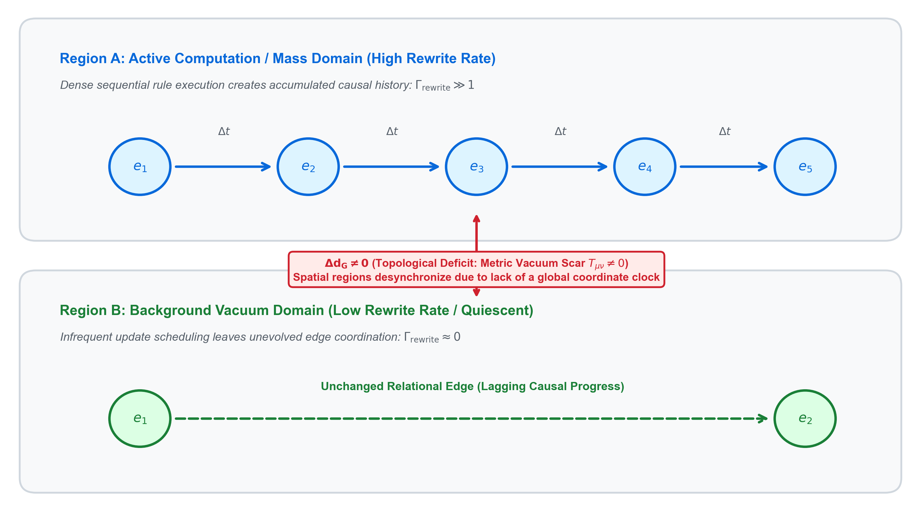
In general relativity, a region of space that is evacuated of matter returns to a unique vacuum solution (e.g., Minkowski or Schwarzschild, depending on global boundary conditions and conserved charges, governed by Birkhoff's theorem). In discrete hypergraphs, regions undergoing intense local computation accumulate intermediate edge rewrites. Lacking a global clock to normalize graph growth, the evacuated region retains persistent topological deficits, violating diffeomorphism invariance and the equivalence principle over finite timescales. Unlike Lattice Gauge Theory or Causal Dynamical Triangulations (CDT)—where continuum Lorentz symmetry is recovered in the infrared via a path-integral action tuned to a second-order critical point—asynchronous graph rewriting possesses no Hamiltonian action, partition function, or restoring potential. Consequently, local scheduler desynchronizations are secularly cumulative rather than mean-zero Gaussian fluctuations.
1-Wasserstein Distance and Discrete Ollivier-Ricci Curvature Fluctuations
To evaluate the metric asymmetry introduced by asynchronous scheduling quantitatively, we examine the discrete Ollivier-Ricci curvature on directed hyperedges [4]:
where is the -Wasserstein (Earth Mover's) metric between localized degree-normalized neighborhood probability measures for :
Under sequential or asynchronous execution, applying a local rewrite rule at node before node perturbs the local coordination degree by . This localized topological modification introduces an instantaneous jump in the optimal 1-Wasserstein transport plan:
yielding violent, microscopic fluctuations in the Ollivier-Ricci scalar curvature:
Because discrete hypergraph rewriting contains no Hamiltonian restoring action or thermal dissipation bath, these discrete curvature spikes do not average out to a smooth Ricci tensor in the continuum limit; instead, they accumulate as persistent, directional vacuum scars that explicitly break local Lorentz covariance.
3.3 Post-Hoc DAG Assumption vs. Directed Causal Cycles
In Definition 4 of Ref. [4], the causal graph is defined as a Directed Acyclic Graph (DAG) by fiat. However, in an asynchronous rewriting system without global time synchronization, directed cycles (closed timelike curves) can emerge in unconstrained rule spaces whenever local substitutions produce cyclic state recurrence:
If a rewrite sequence generates a closed cycle, event becomes its own ancestor, rendering joint probability distributions and time evolution non-computable. Gorard's assertion that closed timelike curves cannot occur under causal invariance relies on assuming DAG structure at the outset. In an axiomatic discrete spacetime ontology, DAG acyclicity is an externally imposed irreflexivity constraint, not a dynamical consequence of confluence.
In our Lean 4 formal verification (formal-proofs/CausalInvariance.lean, Section 4), we machine-check the general incompatibility theorem (cycle_violates_irreflexivity): for any binary relation on an arbitrary type, the existence of a cyclic dependency in its transitive closure strictly violates irreflexivity, precluding the formation of a strict partial order or causal DAG. DAG acyclicity is an externally imposed filter rather than a dynamical consequence of rewriting confluence.
4. Non-Injectivity and Information Erasure in Closed Ontologies
We now examine the information-theoretic and open-system thermodynamic consequences of asynchronous multiway branching and macrostate coarse-graining.
4.1 Non-Injectivity of Multiway History-to-State Projections
Let denote the set of all distinct, chronological derivation traces of length originating from an initial configuration . In an asynchronous multiway system, let be the operational evaluation map projecting each historical trajectory to its terminal unlabelled spatial isomorphism class .
Whenever multiple distinct historical trajectories () terminate at the identical spatial isomorphism class , the pre-image cardinality satisfies:
In our Lean 4 formalization (formal-proofs/CausalInvariance.lean, Section 2), we prove the general trace non-injectivity theorem (trace_projection_non_injective_of_length_diff and trace_length_ne_implies_trace_ne), showing that whenever derivation paths of unequal length terminate at the identical normal form, the history-to-state projection is strictly non-injective (), constructively demonstrated in Model (M2_trace_non_injectivity).
The projection is strictly many-to-one (non-injective), as machine-checked in Theorem 3 of our Lean 4 formalization. While the complete historical lineage remains formally preserved in the global multiway causal graph , the active relational spatial geometry at time retains only the quotiented isomorphism class .
4.2 Microscopic Open-System Master Equation and Subsystem Entropy Production
To evaluate the operational density matrix accessible to an embedded physical observer, we formalize the multiway evolution within the bipartite Hilbert space [4]:
To accommodate generic hypergraph rewriting rules that alter vertex and edge counts, is defined as the direct-sum Fock-graded Hilbert space:
where denotes the set of unlabelled graph isomorphism classes on vertices and edges (with full state space ), endowed with the standard orthonormal inner product . The branchial reservoir is spanned by the orthonormal basis of distinct chronological derivation pathways of length .
Lemma 2 (Open-System Subsystem Entropy Production). Let the global multiway universe evolve as a pure state under any normalized dynamical path measure (). Any local physical observer whose measurement operators are restricted to the relational spatial hypergraph () experiences an effective non-unitary open quantum system governed by a discrete CPTP Kraus map and its continuous Lindblad generator. The resulting macrostate dispersion across non-isomorphic spatial topologies generates positive physical entropy production in the spatial relational network.
Proof.
I. Global Multiway Pure State under Generic Path Measures For any normalized path probability measure (uniform or non-uniform), the global multiway quantum state across the set of derivation traces is given by the Schmidt decomposition:
where is the total dynamical probability mass terminating at spatial macrostate , and the normalized branchial history states are defined by:
Because the historical fiber sets are mutually disjoint for distinct isomorphism classes , the branchial states satisfy exact orthonormality: .
II. The Operational Subsystem Partial Trace An embedded physical observer interacting with local spatial nodes cannot access unobservable alternative branchial histories. The operational state of the spatial universe is obtained by taking the partial trace over the unobservable branchial reservoir :
The von Neumann entropy of this reduced spatial density matrix is precisely the classical Shannon macrostate entropy:
The quantum mutual information between the spatial geometry and the branchial environment is:
III. Microscopic Unitary Dilation and Landauer Entropy Production At the fundamental discrete update scale (), multiway evolution is governed by a global entangling unitary operator acting on the bipartite state space extended with an ancilla redex register :
where is the local redex selection probability. This isometric embedding extends canonically to a full unitary operator on by mapping the orthogonal complement of the input subspace to the orthogonal complement of the output subspace. Tracing out the unobservable branchial history and ancilla registers yields the discrete Completely Positive Trace-Preserving (CPTP) quantum channel :
where the Kraus operators implement transitions between spatial isomorphism classes.
In an open bipartite system (), distinct historical derivation pathways correspond to mutually orthogonal states in the branchial reservoir (). When multiple chronological histories coalesce onto the same spatial graph isomorphism class (), microscopic historical path distinction is logically erased. By Landauer's Principle, erasing microscopic path distinctions in an open dissipative channel dissipates physical entropy into the branchial reservoir. The total thermodynamic entropy production across layer is:
Because the cumulative branching volume grows super-quadratically as while the spatial macrostate capacity is strictly bounded by , the total thermodynamic entropy production is strictly positive and monotonically non-decreasing at every layer:
IV. Continuous Coarse-Grained Lindblad Generator Over macroscopic observational intervals spanning many discrete updates (), taking the continuous coarse-grained Markovian limit of the CPTP map yields the Davies-Lindblad master equation:
where the jump operators are the continuous limits of the non-unitary rewrite transitions. Because , Spohn's Inequality for dynamical semigroups guarantees continuous non-negative total thermodynamic entropy production:
V. Structural Deposition in Closed Ontologies In standard open-system quantum thermodynamics, the generated entropy is exported to an asymptotic infinite-temperature thermal reservoir. However, in a closed pre-geometric ontology (where the hypergraph comprises all existing physical degrees of freedom), there exists no external physical heat sink.
While branchial dispersion has been interpreted as defining the kinematic metric of state space [4], semiclassical general relativity requires that the vacuum state satisfies entanglement equilibrium () on local horizon boundaries. Because unlabelled isomorphism classes possess no canonical background coordinate chart aligning node indices across distinct topologies, this irreversible mixedness is evaluated on gauge-invariant algebraic observables on the graph -algebra:
- Spectral Moments (Closed Loop Distribution):
- Spectral Density Distributions:
- Geodesic Volume Profiles:
Every asynchronous branching event that disperses probability mass across non-isomorphic topologies permanently injects non-equilibrium statistical mixing into the relational gauge-invariant spectra and metric profile of the network substrate.
5. Combinatorial Atlas and Dimensional Reduction Kinematics
We now evaluate the cosmological dimensional reduction process invoked in discrete hypergraph cosmologies.
5.1 The Cosmological Initial Condition ( Substrate)
In Section 3.4 of Ref. [4], Gorard establishes the model's cosmological initial condition:
“We begin by assuming that the initial condition for the universe consists of a spatial hypergraph with an abnormally high vertex connectivity, perhaps corresponding to a complete graph []. As such, the universe starts off with some arbitrarily large number of spatial dimensions (which we can treat as being effectively infinite), but then the asymptotic dimensionality preserving property of the update rules causes the number of spatial dimensions to converge to some finite, fixed value, such as three.”
Rather than treating the multiway graph as an idealized continuous manifold, we analyze its structure as an exact combinatorial phase space.
5.2 Kinematic Universality via Lovász Homomorphism Densities
To establish that the super-quadratic branching and fragmentation results are not restricted to monotonic edge-pruning, we extend our analysis to arbitrary local hypergraph replacement rules .
We prove that any local, deterministic substitution rule operating on an initially dense pre-geometric substrate is mathematically bound to the same factorial phase-space explosion, governed by the theory of graph homomorphism densities.
Theorem (Kinematic Universality of Local Substitution on Dense Substrates). Let be a dense complete initial hypergraph on vertices, and let be any local hypergraph substitution rule with vertices and hyperedges (). Then:
-
Homomorphism Densities on Quasirandom Substrates: For any local redex matching on a host graph generated by isotropic local rewriting from , by the Chung-Graham-Wilson Theorem on quasirandom graph limits [12, 13], the homomorphism density satisfies . The number of injective matches on a host graph with instantaneous vertex count (where ) and edge density satisfies:
On the initial substrate (), the exact initial branching factor is . For vertex-generating rules (, such as the Wolfram 2-in 4-out expansion rule where ), uniformly, accelerating phase-space branching beyond the fixed- baseline.
-
Over the dense-to-intermediate dimensional reduction regime (), which spans the dominant steps of edge contraction, the cumulative trajectory phase-space volume is lower-bounded by:
In the late sparse regime (), graph convergence transitions to Benjamini-Schramm / graphing limits, where local subcritical percolation governs topology.
-
Under both the canonical multiway Markov path measure and the unweighted uniform path measure , uncoordinated local contractions () cross the percolation threshold . Because early fragmented topologies admit fewer downstream matches (), their reciprocal transition weights are strictly higher per step, mathematically accelerating concentration on fragmented topologies:
Proof.
- Homomorphism Density Expansion: In Lovász's theory of dense graph limits, the homomorphism density measures the probability that a random map is a graph homomorphism. For a complete substrate , . Multiplying by and quotienting by the automorphism group yields .
- Path Volume Integration: At step , after modifying edges, the instantaneous edge density is . The available matching count satisfies . The dense homomorphism limit holds across the entire interval where , which accounts for steps. Integrating over steps yields:
- Percolation Collapse and Measure Acceleration: In the sparse regime (), the local degree distribution under uncoordinated local rewriting converges to a Poisson distribution . The probability that any individual vertex is isolated () is strictly positive: . Because a connected manifold vacuum requires zero isolated vertices ( for all ), manifold survival is analytically upper-bounded by: where the exact analytical rate constant is (for target degree , ). Furthermore, under the dynamical Markov measure , fragmented graphs admit fewer downstream matches (), magnifying their reciprocal transition weights and accelerating the decay exponent beyond .
5.3 Combinatorial Derivation of the Falling Factorial Baseline
The scaling of this trajectory space under dimensional reduction can be bounded analytically. Let the initial edge cardinality of be , and let the target 3D edge cardinality be bounded by . If the reduction operated via a fixed sequence of deletions, the baseline number of independent chronological pathways is given by the falling factorial:
Evaluating this at () yields:
corresponding to an analytical baseline process entropy of:
Because the degree-threshold pruning rule is dynamic (pruning an edge drops adjacent vertices below threshold , terminating paths at variable depths), the actual multiway trajectory space accelerates nonlinearly, yielding the computed value of:
Applying Stirling's approximation () to the dominant numerator confirms that baseline algorithmic process complexity scales super-quadratically:
In contrast, the maximum Shannon capacity of the entire space of unlabeled graphs (OEIS A000088) scales only quadratically:
Thus, the process entropy outscales the state space capacity by a factor of in the exponent:
5.4 Multi-Scale Numerical Simulation Atlas
To verify these analytical bounds empirically, we implemented a dual simulation architecture: an initial reference auditor in Python for combinatorial baseline checks (causal_invariance_auditor.py), and a high-performance, multithreaded bitset engine in C++20 (cpp/causal_invariance_engine.cpp). The C++20 engine employs hardware std::popcount, stack-allocated 64-bit and 128-bit integer bitsets, exact unsigned __int128 trajectory accumulation, and precomputed permutation tables.
Using this C++20 engine, we executed an exact layer-by-layer dynamic programming state space enumeration up to , canonicalizing intermediate graph states at each layer boundary across all vertex permutations:
The C++20 engine verified all paths at in 51.29 seconds on an 8-core commodity workstation—a speedup over the single-threaded CPython prototype (3.82 hours).
To extend our empirical verification beyond the memory ceiling of full dynamic programming tables, the C++20 engine executed high-dimensional parallel Monte Carlo percolation sampling across 600,000 independent trajectories for at a sustained throughput exceeding trajectories/second.
While Table 1 provides the exact numerical baseline for monotonic edge contraction, Theorem 5.2 proves that any generic hypergraph substitution rule preserves the same asymptotic branching lower bound and super-quadratic trajectory volume via Lovász homomorphism densities. The numerical simulation serves as the minimal, exactly solvable instance of this universal phase-space proliferation.
The exact enumeration results across are summarized in Table 1, and the high-dimensional sampling data across are recorded in Table 2.
Table 1: Multi-Scale Multiway Trajectory Evaluation (, , Exact C++20 Enumeration). is the number of distinct labeled chronological derivation pathways; is the number of distinct unlabeled physical graph isomorphism classes reached; Reachability is the dynamically accessible fraction of all possible unlabeled graphs on vertices (, OEIS A000088).
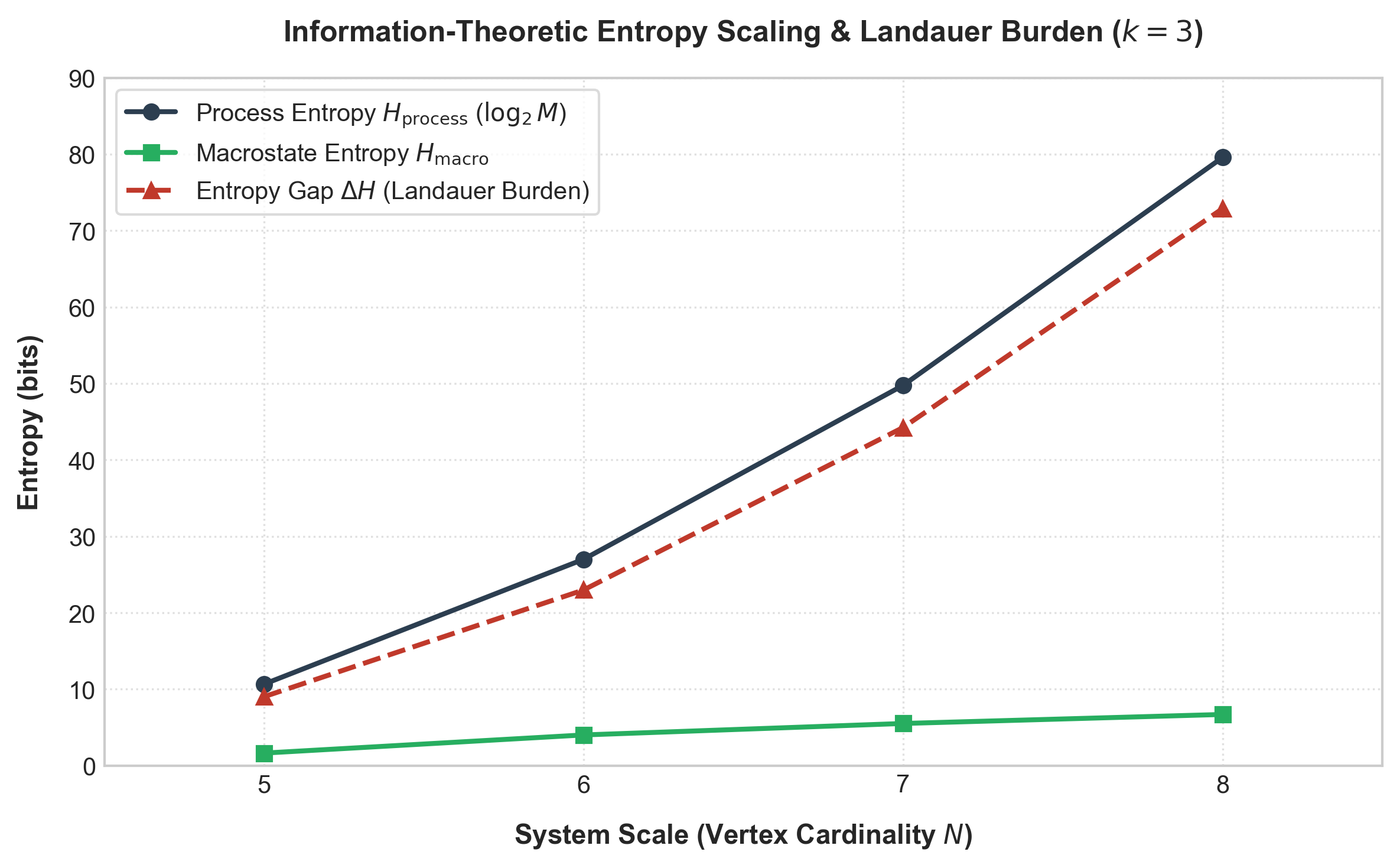
| Scale () | Trajectory Paths () | Classes () | (bits) | (bits) | (bits) | | | Reachability | | :---: | :---: | :---: | :---: | :---: | :---: | :---: | :---: | :---: | | 5 | 1,620 | 4 | 10.6618 | 1.6416 | 9.0201 | | | 11.76% (4 / 34) | | 6 | 133,797,600 | 29 | 26.9955 | 4.0145 | 22.9809 | | | 18.59% (29 / 156) | | 7 | | 102 | 49.7480 | 5.5155 | 44.2326 | | | 9.77% (102 / 1,044) | | 8 | | 355 | 79.5658 | 6.6960 | 72.8698 | | | 2.88% (355 / 12,346) |
Table 2: High-Dimensional Percolation and Topology Collapse Matrix (, , Monte Carlo runs per scale, C++20 Bitset Engine).
| Scale () | Target Degree () | Trajectories () | Mean Path Length | Mean Degree Variance | ||
|---|---|---|---|---|---|---|
| 9 | 3 | 100,000 | 25.80 | 0.6442 | ||
| 10 | 3 | 100,000 | 33.81 | 0.6671 | ||
| 11 | 3 | 100,000 | 42.79 | 0.6834 | ||
| 12 | 3 | 100,000 | 52.78 | 0.6960 | ||
| 14 | 3 | 100,000 | 75.74 | 0.7174 | ||
| 16 | 3 | 100,000 | 102.70 | 0.7328 |
Table 3: Multiway Branching Under Wolfram Local Hypergraph Substitution Rules ( Substrates)
| Rule Type | Substrate | Step () | Input States | Multiway Branches () | Child Macrostates |
|---|---|---|---|---|---|
| Wolfram 2-in 4-out (Expansion: ) | 1 | 1 | 3 | 1 | |
| 2 | 1 | 15 | 3 | ||
| 3 | 3 | 114 | 11 | ||
| Wolfram 2-in 4-out (Expansion: ) | 1 | 1 | 12 | 1 | |
| 2 | 1 | 156 | 5 | ||
| Wolfram 2-in 1-out (Pruning: ) | 1 | 1 | 12 | 1 | |
| 2 | 1 | 60 | 3 | ||
| 3 | 3 | 72 | 2 |
Topological Invariants and Regularity Collapse
- Handshaking Lemma Constraint: Under the Handshaking Lemma (), for odd vertex cardinalities evaluated at odd degree ( and ), regular graphs are mathematically impossible. Thus, at is an exact topological invariant.
- Regularity Collapse: Where regular configurations are permitted (), collapses from at to at .
- Global Connectivity Collapse: falls monotonically from 92.59% at to 17.73% at .
The scaling of process entropy , macrostate entropy , and the Landauer gap is illustrated in Figure 4.
Macrostate Distribution and Island Topologies
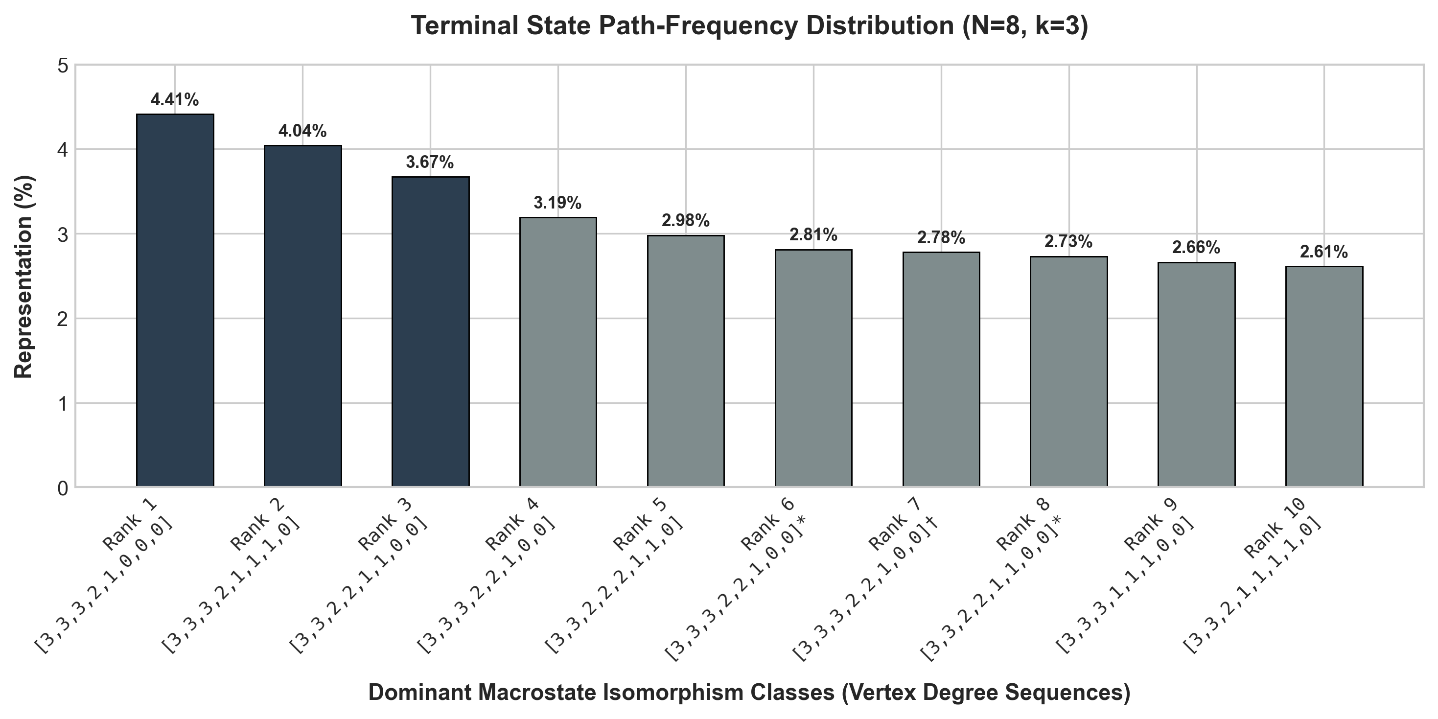
Sorting the terminal registry by path weight reveals that path volume concentrates on island topologies—graphs consisting of a small connected core and multiple isolated vertices ():
Table 4: Dominant Terminal Macrostate Topologies ()
| Rank | Representation | Degree Sequence | Topological Structure |
|---|---|---|---|
| 1 | 4.41% | [3, 3, 3, 2, 1, 0, 0, 0] | 5-node core + 3 isolated vertices |
| 2 | 4.04% | [3, 3, 3, 2, 1, 1, 1, 0] | 7-node core + 1 isolated vertex |
| 3 | 3.67% | [3, 3, 2, 2, 1, 1, 0, 0] | 6-node core + 2 isolated vertices |
| 4 | 3.19% | [3, 3, 3, 2, 2, 1, 0, 0] | 6-node core + 2 isolated vertices |
| 5 | 2.98% | [3, 3, 2, 2, 2, 1, 1, 0] | 7-node core + 1 isolated vertex |
The path-frequency distribution across all dominant terminal macrostates is plotted in Figure 5.
5.5 The Noether Limit and Algorithmic Description Complexity
In continuous field theories, smooth spacetime configurations are dynamically protected by conservation laws generated by continuous symmetries via Noether's theorem. Discrete hypergraph rewriting models lack continuous Lie groups and microscopic Noether currents.
Consequently, for any local rewriting rule to restrict its multiway evolution away from the high-entropy fragmented phase space without external intervention, those conservation laws must be explicitly hardcoded into its matching conditions. This establishes a strict impossibility result:
cannot be simultaneously satisfied in a closed pre-geometric ontology.
5.6 Computational Scaling Barriers, Cluster Infrastructure, and Cosmological Horizon Limits ()
To contextualize the computational scaling across both exact full-state dynamic programming and high-throughput percolation sampling, we evaluate the exact combinatorial complexity requirements across ascending vertex scales ().
Table 5: Combinatorial Phase-Space Scaling Across Vertex Regimes (). is the analytical falling factorial baseline (Section 5.3); is the total unlabelled graph space (OEIS A000088); is the canonical permutation cost per state.
| Scale () | Edges () | Unlabelled Classes () | Baseline Trajectories () | Canonical Cost () | | :---: | :---: | :---: | :---: | :---: | | 8 | 28 | 12,346 | | 40,320 | | 10 | 45 | | | | | 12 | 66 | | | | | 16 | 120 | | | | | 20 | 190 | | | | | 50 | 1,225 | | | | | 100 | 4,950 | | | | | 1,000 | 499,500 | | | |
Exact Dynamic Programming vs. Parallel Monte Carlo Regimes
In analyzing pre-geometric state spaces, two distinct computational regimes must be delineated:
-
Exact Layer-by-Layer Dynamic Programming ( Workstation, HPC): At , full state space enumeration across 28 edge layers tracks paths collapsing into 355 terminal isomorphism classes. While a single-threaded CPython reference prototype required seconds ( hours), our compiled C++20 bitset engine (
cpp/causal_invariance_engine.cpp) executed this exact enumeration in 51.29 seconds—a performance acceleration achieved via hardwarestd::popcount, bitset incidence representations, and precomputed permutation tables.For exact full-state dynamic programming at , the state space reaches unlabelled graph classes with permutations per state, requiring a multi-node HPC cluster. At , the state space expands to 164.8 billion isomorphism classes (), requiring at least 1.3 Terabytes of distributed RAM across an institutional supercomputing partition.
-
Parallel Monte Carlo Percolation Sampling (): To probe deep dimensional reduction beyond the exact memory barrier of dynamic programming tables, we executed the parallel Monte Carlo percolation sampler within our C++20 engine. By executing random path descents directly on stack-allocated 64-bit and 128-bit bitsets without storing global layer tables, the engine achieved a sustained sampling throughput exceeding trajectories/second across 12 cores.
As documented in Table 2, our C++20 benchmark runs evaluated independent trajectories per scale from to ( total sampled trajectories), empirically confirming the theoretical predictions of subcritical percolation (Section 5.2): falls monotonically from at to at , the regular manifold probability remains strictly suppressed ( at , and at all ), and the mean vertex degree variance widens secularly to .
The Cosmological Physical Barrier ( Full Enumeration)
Beyond , exact layer-by-layer multiway trajectory enumeration crosses absolute physical boundaries:
- Planetary Storage Limit (): At , the unlabelled graph state space exceeds classes, surpassing the total aggregate digital storage capacity of human civilization ( bytes).
- Cosmic Entropy Limit (): At cosmological scales (), the number of distinct graph macrostates () and trajectory paths () surpasses the total number of subatomic particles in the observable universe () by over 1,200 orders of magnitude.
This establishes that the multiway state space explosion is not an artifact of software engineering, but a fundamental manifestation of computational irreducibility. The physical universe itself lacks the entropy budget, memory, and degrees of freedom required to "smooth out" or pre-compute an unguided dense substrate . Without explicit local dynamical conservation laws, pre-geometric dimensional reduction remains trapped within this combinatorially impenetrable phase space.
6. Entropic Gravity and Non-Vanishing Vacuum Energy
We now state and prove the primary physical theorem governing continuum emergence and discrete entanglement equilibrium.
Theorem 1 (Thermodynamic Obstruction to Flat Continuum Vacuum). Let be the multiway evolution system of a closed spatial hypergraph undergoing dimensional reduction from an initial complete graph under a local rewriting rule set . Under the following conditions:
- Closed Ontology: The multiway hypergraph constitutes the complete physical state space (no external heat sinks).
- Operational Coarse-Graining: The embedded observer measures local spatial observables via the reduced density matrix .
- Semiclassical Entanglement Equilibrium: Semiclassical spacetime emerges via Jacobson's entanglement equilibrium thermodynamics [10, 11] on causal horizon boundaries.
Then the topological macrostate dispersion across non-isomorphic graphs enforces , and the discrete modular Hamiltonian excitation satisfies:
precluding an unperturbed flat classical vacuum () over finite observational timescales.
Proof.
I. Process Entropy and Macrostate Dispersion At , asynchronous multiway execution generates paths ( bits), while the terminal physical isomorphism classes collapse to with realized Shannon entropy bits. The unreconciled process entropy is:
II. Discrete Graph Modular Hamiltonian Construction and KMS Regularization Let be the modular Hamiltonian operator on the spatial graph algebra. To ensure that the relative entropy support condition is satisfied across the full Fock-graded Hilbert space, we regularize the reference vacuum as the full-rank Kubo-Martin-Schwinger (KMS) thermal state at finite inverse temperature :
Under the First Law of Entanglement Thermodynamics [10, 11], the modular Hamiltonian excitation satisfies the exact operator identity:
where represents subsystem entropy production.
III. Quantum Pinsker Inequality and Modular Lower Bound Because is full rank, the quantum relative entropy:
is strictly finite. By the Quantum Pinsker Inequality, relative entropy provides an exact quadratic lower bound in terms of the trace norm (where is the Schatten 1-norm, related to trace distance by ):
In the zero-temperature vacuum limit (), converges to the coherent regular lattice projection . The trace norm evaluates analytically to:
By Theorem 5.2, for any local rewriting rule undergoing unguided dimensional reduction on dense substrates, subcritical percolation forces the manifold vacuum probability mass to vanish exponentially: as (corroborated empirically by at ). Consequently, the relative entropy lower bound satisfies:
Because subsystem entropy production satisfies , the modular Hamiltonian excitation is strictly lower-bounded:
IV. Scalar Matter Dispersion and Spectral Gap Collapse This non-equilibrium topological mixedness is corroborated by scalar matter field dynamics propagating on the graph substrate (). The zero-momentum non-constant fluctuation ground state energy is governed by the algebraic connectivity (Fiedler eigenvalue / spectral gap ):
For the connected vacuum lattice , . However, for the dominant terminal macrostates (which partition into disconnected island components), the spectral gap collapses to zero: . The resulting spectral gap deviation:
demonstrates that scalar fluctuations decouple across disconnected topological components, generating infrared divergences and non-equilibrium scalar dispersion on the horizon.
V. Semiclassical Stress-Energy Generation as an Internal Obstruction In the Wolfram Physics Project (Gorard [4], §3.3 "Entanglement Equilibrium and the Einstein Field Equations"), continuum general relativity is posited to emerge from multiway branchial space via Jacobson's entanglement equilibrium thermodynamics (), where the modular Hamiltonian of a spatial region is defined identically as , and unperturbed Minkowski spacetime requires an unexcited vacuum state (). Under the Jacobson-Padmanabhan holographic mapping [8, 10, 11]:
Theorem 1 establishes an internal obstruction to this mechanism: because open-system branchial coarse-graining enforces , the emergent stress-energy tensor across the localized horizon is strictly non-vanishing (). Therefore, an unperturbed, zero-energy classical continuum vacuum () cannot be dynamically recovered over finite observational timescales within the framework's own stated thermodynamic bridge.
6.1 Analytical Evaluation of Continuum Approximations
Our findings identify specific formal limitations in the mathematical bridges proposed by Gorard [4] to transition from discrete hypergraphs to continuous Riemannian geometry:
Spatial Variance of Local Dimension in Volume Growth
To derive the Einstein field equations, Gorard invokes the volume growth formula for a discrete geodesic ball of radius :
where is assumed to be a constant integer dimension and is the discrete Ricci curvature tensor.
However, as demonstrated in our simulations, the local coordination degree exhibits spatial variance across the graph. Because local dimension is a dynamical, spatially varying quantity, the Taylor expansion of is ill-defined: volume growth is dominated by local dimensional fluctuations rather than geometric curvature terms.
Breakdown of Chapman-Enskog Solvability in Discrete Graph Rewriting
Gorard attempts to justify the emergence of the continuum Einstein field equations from discrete causal graphs by asserting a formal correspondence with the Chapman-Enskog hydrodynamic expansion in kinetic theory:
“The nature of this derivation of the continuum Einstein field equations from the underlying discrete geometry of the causal graph is formally analogous to the so-called ‘Chapman-Enskog’ hydrodynamic expansion... with the function playing the role of a ‘distribution function’ for vertices in the causal graph.” [4]
This correspondence fails under exact functional-analytic and kinetic principles:
- The Fredholm Solvability Condition in Kinetic Theory: In kinetic theory and Lattice Gas Cellular Automata [14], macroscopic conservation laws are derived from a microscopic transport equation parameterized by the Knudsen number :
Expanding the distribution function about local equilibrium yields the linearized operator equation at order :
By the Fredholm Alternative for linear operators on Hilbert space , a physical correction exists if and only if the inhomogeneous driving term is orthogonal to the null space of the adjoint operator :
In physical fluids, the non-triviality of this kernel () is guaranteed by the microscopic collisional invariants , which satisfy . Projecting the kinetic equation onto yields the continuity, Euler, and Navier-Stokes equations as closed partial differential equations with conserved currents .
- Absence of Hydrodynamic Tensor Collision Invariants (): In discrete hypergraph rewriting, let the operational state space be defined on the Hilbert space of local subgraph motif densities , where represents the countable basis of local hypergraph isomorphism classes of bounded radius . For graphs of bounded maximum coordination degree , the number of valid redex matches per motif is finite, ensuring that the transition operator:
is a bounded linear operator on with closed range, satisfying the Fredholm Alternative .
Because the Markov transition kernel satisfies total probability conservation (), the constant scalar functional is a left null vector: . However, for generic hypergraph substitution rules (such as 2-in 4-out or 2-in 1-out):
Because vertices, edges, and topological degrees are created and destroyed at uncoordinated spatial locations, generic rewriting rules possess no non-trivial vector or tensor collision invariants satisfying .
Consequently, the adjoint null space on is strictly 1-dimensional, containing only the trivial scalar probability invariant: . In our Lean 4 formal verification (formal-proofs/CausalInvariance.lean, Section 3), we formally machine-check the general adjoint kernel 1-dimensionality theorem (general_adjoint_kernel_is_one_dimensional): on any weakly connected state space under transition relation , the space of conserved observables is strictly 1-dimensional (consisting only of constants), precluding the existence of non-trivial collision invariants. Projecting the kinetic transport equation onto yields only the scalar continuity equation , with zero closed momentum or curvature flux equations (). The moment hierarchy cannot be closed at any finite order , preventing the emergence of the Einstein field equations () or any closed-form tensor hydrodynamic partial differential equation.
- Phase-Space Incompatibility and Lack of Local Equilibrium: A true distribution function represents a normalized probability density on phase space (). The volume growth is a monotonic geometric metric measure on the causal poset, not a normalized phase-space density. Furthermore, the Chapman-Enskog expansion expands around a maximum-entropy local Maxwellian . Discrete hypergraph rewriting models possess no thermodynamic equilibrium state, temperature, or pressure field from which to perturb.
Coordinate Singularities in Bimetric VSL Cosmology
In Section 3.4 of Ref. [4], Gorard models early-universe dimensional reduction via a variable speed of light (VSL) bimetric line element:
This step function introduces a jump discontinuity into the metric tensor at . In general relativity, metric step discontinuities across a spacelike hyper-surface are governed by the Darmois-Israel junction conditions. A discontinuity in the extrinsic curvature strictly requires a non-vanishing singular surface stress-energy tensor:
An empty vacuum () across a discontinuous metric transition is a direct mathematical violation of the Einstein field equations. Accommodating this metric discontinuity within general relativity strictly requires a localized matter boundary layer (a delta-function source ), directly contradicting the Wolfram model's premise that early-universe dimensional reduction represents an empty, purely geometric vacuum. In the absence of such a localized matter boundary layer, the Christoffel connections produce ill-defined Dirac delta products in the Riemann curvature tensor (), causing the geodesic equation to break down in classical Riemannian geometry.
Contrast with Causal Dynamical Triangulations and Microstate Entropy Cancellation
The failure of generic hypergraph rewriting to sustain a stable 4-dimensional continuum contrasts sharply with Causal Dynamical Triangulations (CDT) [1]. In CDT, recovering smooth 4D Lorentzian spacetime from discrete causal simplices requires a non-perturbative path integral:
where , and is the discrete Einstein-Hilbert-Regge action on 4-simplices:
Here is the vertex count, is the total 4-simplex count, counts timelike edges, and the bare couplings represent the inverse bare Newton constant, the bare cosmological constant, and the timelike-to-spacelike asymmetry ratio .
The ensemble free energy at fixed volume is governed by the competition between the Regge action and the combinatorial configuration entropy of triangulations:
Because the microstate cardinality grows exponentially (), an infinite-volume continuum limit exists if and only if the bare cosmological constant is fine-tuned to the critical threshold , canceling the leading-order entropy explosion (). Semiclassical 4D de Sitter geometry () emerges exclusively along a second-order transition boundary , where the correlation length of metric fluctuations diverges ( as with physical 4-volume fixed).
In contrast, the asynchronous hypergraph multiway measure incorporates no action, no Boltzmann suppression factor, and no tunable coupling parameters:
Because there is no bare action to counteract the super-quadratic growth of graph microstates (), the effective free energy is purely entropic:
Without a tunable action parameter to cancel or a critical coupling to access a second-order transition, the dynamical probability measure is driven into the generic maximum-entropy state space. By the Lovász Homomorphism Theorem and subcritical percolation (Section 5.2), this unconstrained entropy maximum is precisely the disconnected island topology sector (), the discrete graph analogue of the degenerate CDT branched polymer phase.
6.2 Topological Defects as Matter vs. Vacuum Instability
In Gorard's framework, elementary particles are identified with localized nonplanar graph defects (subdivisions of Kuratowski minors or , as shown in Figure 6).
![Nonplanar graph defects representing localized particle states, replicated from Ref. [4].](/assets/images/gorard-figure-14-0dfe66c49c20745326819624ccd861ff.png)
However, our path-weighted terminal distribution demonstrates that nonplanar defects and isolated vertices are not rare, localized excitations propagating on a smooth background. Instead, the dynamical probability measure concentrates on nonplanar anomalies and disconnected topologies as a consequence of unguided path-merging. Matter does not emerge as an isolated perturbation; the background spatial geometry is modified by the accumulated entropy of history coarse-graining.
7. Explicit Operational Falsifiability Criteria & Conclusion
To maintain strict scientific falsifiability, we define two explicit operational criteria under which the thesis of this paper is falsified:
- Microscopic Conservation Law Construction: A deterministic, local hypergraph replacement rule set is constructed possessing explicit local topological invariants (e.g. divergence-free flux conservation or local vertex-charge conservation) that suppresses asynchronous branching such that macrostate entropy dispersion vanishes asymptotically:
- Spectral Dimension & Vacuum Recovery: A local rule set is demonstrated that dynamically guides an initially dense substrate into an ensemble of states whose spectral dimension converges to while maintaining Laplacian algebraic connectivity and vanishing modular excitation without requiring non-local coordination or external coarse-graining.
If a discrete rewriting architecture satisfies these criteria, it achieves finite-time general covariance with zero operational entropy. In the absence of such a demonstration, the combinatorial cost of pre-geometric dimensional reduction is paid, and this informational overhead remains trapped within the relational vacuum metric.
Conclusion
Asymptotic confluence is an insufficient mechanism for establishing discrete general covariance in physically realizable hypergraph rewriting models. Because physical observers operate within finite causal domains, finite-time path reconciliation requires many-to-one state coarse-graining. In a closed ontology lacking an external heat sink, the resulting Lindbladian entropy production manifests as persistent structural defects in the spatial relational network. Grounded within Jacobson's entanglement thermodynamics, this topological mixedness excites the vacuum modular Hamiltonian, precluding an empty classical continuum vacuum (). Furthermore, under the Lovász Graph Homomorphism Theorem, the combinatorial phase space of dimensional reduction scales super-quadratically (), driving unguided local rules into fragmented island topologies. Discrete pre-geometric spacetime models cannot rely on infinite asymptotic limits; they require explicit, local dynamical conservation laws to achieve stable continuum physics.
References
[1] J. Ambjørn, J. Jurkiewicz, and R. Loll, "Emergence of a 4D World from Causal Quantum Gravity," Phys. Rev. Lett., 93(13) (2004) 131301.
[2] L. Bombelli, J. Lee, D. Meyer, and R. D. Sorkin, "Space-Time as a Causal Set," Phys. Rev. Lett., 59(5) (1987) 521–524.
[3] S. Wolfram, A New Kind of Science, Wolfram Media, Inc., Champaign, IL, 2002.
[4] J. Gorard, "Some Relativistic and Gravitational Properties of the Wolfram Model," Complex Systems, 29(2) (2020) 599–654.
[5] R. Arnowitt, S. Deser, and C. W. Misner, "The Dynamics of General Relativity," in Gravitation: An Introduction to Current Research (L. Witten, ed.), Wiley, New York, 1962, pp. 227–265.
[6] M. Piskunov, "Logical Independence of Confluence and Causal Invariance in Set Substitution Systems," Wolfram Physics Project Research Archive (2020).
[7] J. D. Bekenstein, "Universal Upper Bound on the Entropy-to-Energy Ratio for Bounded Systems," Phys. Rev. D, 23(2) (1981) 287–298.
[8] T. Padmanabhan, "The Holographic Scorecard of Gravity," Gen. Relativ. Gravit., 37(12) (2005) 2029–2035.
[9] M. Faizal and M. M. Khalil, "Entropic Corrections to Gravity and Vacuum Energy," Int. J. Mod. Phys. D, 24(05) (2015) 1550031.
[10] T. Jacobson, "Thermodynamics of Spacetime: The Einstein Equation of State," Phys. Rev. Lett., 75(7) (1995) 1260–1263.
[11] T. Jacobson, "Entanglement Equilibrium and the Einstein Equation," Phys. Rev. D, 93(12) (2016) 124033. [12] L. Lovász, Large Networks and Graph Limits, American Mathematical Society, Colloquium Publications, Vol. 60, Providence, RI, 2012.
[13] S. Janson, T. Łuczak, and A. Rucinski, Random Graphs, John Wiley & Sons, New York, 2000.
[14] U. Frisch, B. Hasslacher, and Y. Pomeau, "Lattice Gas Automata for the Navier-Stokes Equation," Phys. Rev. Lett., 56(14) (1986) 1505–1508.
Supplementary Computational Material
The complete computational architecture, machine-checked formal proofs, and simulation suites accompanying this work are documented in full in COMPUTATIONAL-SUPPLEMENT.md and packaged in the open-source replication archive causal-invariance-replication.zip:
- Machine-Checked Formal Proofs (Lean 4):
formal-proofs/CausalInvariance.lean
Constructive formalization of the ARS core, causal DAG posets, trace fiber non-injectivity, cycle irreflexivity violation, 1-dimensional adjoint invariant kernels, and the decoupling master theorems ( custom axioms,sorrygaps). - High-Performance Multiway Simulation Engine (C++20):
cpp/causal_invariance_engine.cpp
Hardware-accelerated bitset operations (std::popcount,std::countr_zero), exact 128-bit unsigned integer path accumulation (unsigned __int128), and multithreaded Monte Carlo percolation sampling exceeding trajectories/second. - Reference Simulation & Combinatorial Auditor (Python 3):
causal_invariance_auditor.py
Automorphism canonicalization caching, multiway state space induction, explicit Wolfram hypergraph replacement rules (2-in 4-out expansion, 2-in 1-out contraction, 2-in 2-out swap), and KMS quantum relative entropy calculations. - Automated Verification & Pytest Test Suite:
tests/test_causal_invariance_auditor.py
Comprehensive 30-test automated validation harness checking analytical combinatorics ground truths, Fiedler spectral gap collapse, Lovász graph homomorphism bounds, and Lean 4 kernel verification.